| |
| Tariff
A B A&B
| |
| Expansion
A B A&B
|

| Variants:
Inelastic Demand by ...
| |
| Country A | |
| Equil. | Tariff |
| Country B | |
| Equil. | Tariff |
| Both | |
| Equil. | Tariff |
| Both Very Inelastic | |
| Equil. | Tariff |
|

|
| ||||||||||||||||||||||||||
|
|
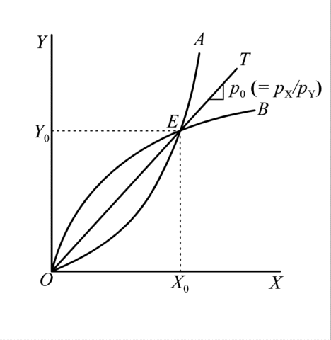
The offer curve OA records the quantities of good X that country A supplies to the world market for export and the quantities of good Y that it demands from the world market as imports, for all prices. The prices are only implicit in the diagram, represented as rays from the origin the slopes of which are the prices of good X relative to good Y. This is possible since balanced trade (which is assumed throughout), requires that pY Y = pX X, and therefore that Y/X = pX / pY . Thus the offer curve can be read as giving the quantity of good X that country A is willing to export in exchange for various quantities of imported good Y, or equivalently as the amounts of both X and Y that it is willing to trade at various prices along rays from O.
Offer curve OB is similarly defined for country B, except that the directions of trade for it are reversed. This is why it is something of a mirror image of OA. That is, it records quantities of good Y that B will export in exchange for various quantities of imports of good X. In equilibrium, of course, country B must import what A exports and vice versa, which is why equilibrium is found where the two curves intersect, at E.
By representing both good X and good Y in a single diagram in this way, the intersection of the two offer curves depicts equilibrium in both markets simultaneously, something that is possible (indeed necessary) because of Walras' Law.
Offer curves need not be upward sloping throughout. If they are, as drawn in the basic picture above, that says that the country is willing to spend more, in exports, for additional quantities of imports as their price falls (and the relative price of exports therefore rises). If this is true, it means that the demand for imports is elastic, and therefore such offer curves are often themselves called "elastic." If demand for imports instead becomes inelastic at low import prices -- which is possible but not theoretically necessary -- then the offer curve bends back on itself as shown in the variants above. This, as the pictures show, can lead to different sorts of responses of prices and quantities of trade to various shocks.
| Tariff | |
|
The effects of a tariff on a country's offer curve depend on how the tariff revenue is spent. If, as is customary to assume, it is redistributed, then the tariff in a nondistorted economy unambiguously reduces the desired quantities traded at any given world price. Thus the offer curve shifts in toward the origin along every ray. Beyond this, one cannot say much about the size of the shift, which depends on both preferences and the constraints of technology and factor endowments. Nonetheless, this is often enough to determine qualitatively the effects on equilibrium prices and quantities, at least on the world market.
As shown in the figures above, with both offer curves elastic a tariff by either country (or both) reduces the quantities of both goods traded. The effect on the world price (terms of trade) depends (not necessarily simply) on the sizes of the two tariffs, each country's terms of trade tending to improve most the larger is its own tariff and the smaller is the other country's. This, of course, is the reason for the likelihood of retaliation when a country seeks to use an optimal tariff. | |
| Expansion | |
|
Economic expansion, due either to factor accumulation or technological progress, tends to cause a country to trade more at any given prices, and thus shifts its offer curve out away from the origin. This is not inevitable, however, as illustrated elsewhere with the trade and transformation curve diagram, which shows that if expansion is sufficiently biased in favor of the import-competing good, desired trade may decrease. The figures above, however, all assume that economic expansion in a country causes it to trade more, for given prices.
The outward shift of a country's offer curve that results is therefore just the opposite of the inward shift due to a tariff, although the exact shape of the change could well be different. Not much more therefore needs to be said about this case. | |
| Variants | |
|
Implications of a tariff (and of expansion, for that matter) can be somewhat different when import demands are inelastic than when they are elastic, as the variants shown above illustrate. For a country that levies a tariff, having its own import demand be inelastic does not matter a great deal, except perhaps to the sizes of the changes that result. But having the foreign offer curve be inelastic matters a lot.
When country A levies a tariff against a world whose demand for its export is inelastic, then the effect is actually to increase its quantity of imports, not reduce it. The reason is that by reducing its demand for imports at the initial price it causes the price of its imports to fall and of its exports to rise. But the inelastic foreign demand means that the other country increases its expenditure on imports when their price rises, and their expenditure is their exports. So the price of their exports must fall by enough to induce the tariff-levying country to buy more of them. Get that? Things seem to get even stranger if both countries have inelastic import demands, especially in the extreme case shown at the bottom right above. Here, almost everything seems to go nuts, as country A's tariff seems to cause it to push up the price of its imports and down the price of its exports, therefore causing it to export more and import less. This appearance is deceiving, however, for all of this weirdness started from an equilibrium that, on inspection, would have been unstable. In the unlikely event that the world started from the unstable equilibrium at E in the bottom right figure, the tariff would actually have caused the system to move to the stable equilibrium northwest of it, with results much more like the other cases. | |