The empirically based Monod growth rate equation ![]() has become popular, compared to the other proposed rate equations for cell
growth, due to its similarity with the mechanistically derived Michaelis-Menten rate law
has become popular, compared to the other proposed rate equations for cell
growth, due to its similarity with the mechanistically derived Michaelis-Menten rate law ![]() for enzyme-catalyzed reaction rate. The Monod
equation is capable of explaining or simulating the exponential growth phase followed by the decelerating growth
phase in the cell concentration during batch growth dynamics, when coupled with dynamic balance equation for the
substrate concentration:
for enzyme-catalyzed reaction rate. The Monod
equation is capable of explaining or simulating the exponential growth phase followed by the decelerating growth
phase in the cell concentration during batch growth dynamics, when coupled with dynamic balance equation for the
substrate concentration:

where YC/S is the stoichiometric yield coefficient of grams of cell mass produced from a gram of substrate.

Figure 1. Typical growth phases in batch cultures of bacterial cells
The initial lag and accelerating growth phases which are not simulated by the Monod growth rate equation can be easily simulated by making a slight modification to the original Monod equation given above. This modification invokes a rate-limiting enzyme involved in the growth processes that may not be present at sufficient levels in the inoculum or starting culture. While cell growth is a complex process mediated by thousands of enzymes, it may be sufficient to hypothesize just a single enzyme that may be rate-limiting during the initial lag growth phase for the purpose of simulating the lag.
Incorporating the effect of varying key enzyme concentration into the Monod growth kinetics, we can write
![]() (R.7.4.3)
(R.7.4.3)
where ER represents the relative amount of the key enzyme in the cell. This modified Monod rate equation follows the Michaelis-Menten rate equation closely, which is more correctly written as
![]() (R.7.4.4)
(R.7.4.4)
where ET represents the total enzyme concentration in the reaction mixture.
Relative key enzyme content inside the cells, ER, may be written as
![]() , where e is the intracellular
content of the key enzyme, with the units of g enzyme/g cell mass, and emax is is the maximum
enzyme concentration in the cell, also with units of g enzyme/g cell mass. The balance equation for the
intracellular enzyme content can be written in terms of eCc, which has the units of g
enzyme/culture volume, as
, where e is the intracellular
content of the key enzyme, with the units of g enzyme/g cell mass, and emax is is the maximum
enzyme concentration in the cell, also with units of g enzyme/g cell mass. The balance equation for the
intracellular enzyme content can be written in terms of eCc, which has the units of g
enzyme/culture volume, as
![]() (R.7.4.5)
(R.7.4.5)
where a and b are enzyme synthesis and degradation rate constants. Using the product rule, we can expand the above equation to write the balance equation for e as:
![]() (R.7.4.6)
(R.7.4.6)
The last term in the above balance equation for the intracellular enzyme is the dilution term due to cell growth, which will be obtained similarly for all intracellular species. This equation can be solved to produce the curve added at the bottom of the batch growth dynamics as shown in Figure 2. The maximum level of the intracellular enzyme emax can be determined easily by setting the above equation to zero and solving for its steady state value. In terms of the model parameters, the maximum level of intracellular enzyme obtained during the exponential growth phase (when Cs is much greater than Ks) can be derived as
![]() (R7.4.7)
(R7.4.7)
Starting with a low or zero content of the key enzyme needed for growth on a given substrate (representative of poor quality starter culture or inoculum), the presence of the substrate induces the synthesis of the key enzyme. The low or zero enzyme content causes the initial lag phase of no cell growth while increasing enzyme content results in the accelerating growth phase. The enzyme concentration reaches and stays at its maximum, emax, during the exponential growth phase, which shows up as a linear increase in the logarithmic plot of cell concentration. The slope of this line on the semi-logarithmic plot below is the maximum specific growth rate, mmax . As the substrate gets depleted, the growth rate or the slope of this curve decelerates and becomes zero when the substrate is completely consumed. With the substrate no longer present, the key enzyme synthesis stops and enzyme degradation during the stationary and death phases reduces the intracellular enzyme content to low levels.
POLYMATH code:
Calculated values of the DEQ variables
Variable initial value minimal value maximal value final value
t 0 0 4 4
Cc 0.1 0.1 1.7 1.7
Cs 4 8.83E-11 4 8.83E-11
e 8.3E-05 8.3E-05 1.05E-04 1.02E-04
Ycs 0.4 0.4 0.4 0.4
alpha 1.0E-04 1.0E-04 1.0E-04 1.0E-04
beta 0.05 0.05 0.05 0.05
mumax 0.9 0.9 0.9 0.9
Ks 0.1 0.1 0.1 0.1
emax 1.053E-04 1.053E-04 1.053E-04 1.053E-04
ER 0.7885 0.7885 0.9975504 0.9686493
mu 0.6923415 7.698E-10 0.8642779 7.698E-10
ODE Report (RKF45)
Differential equations as entered by the user
[1] d(Cc)/d(t) = mu * Cc
[2] d(Cs)/d(t) = -1/Ycs * mu * Cc
[3] d(e)/d(t) = alpha * Cs/(Ks + Cs) - beta*e - mu*e
Explicit equations as entered by the user
[1] Ycs = .4
[2] alpha = .0001
[3] beta = .05
[4] mumax = .9
[5] Ks = .1
[6] emax = alpha/(mumax+beta)
[7] ER = e/emax
[8] mu = mumax * ER*Cs/(Ks + Cs)

Figure 2. Dynamic profiles of substrate concentration and intracellular enzyme content along with the logarithm of cell mass concentration.
Click here for the Polymath Code
Consider the cell growth medium in a batch bioreactor that contains two different carbon substrates, S1 and S2, which are each capable of supporting cell growth. For the growth on the substrate 1:
Cells + Substrate 1 (e.g. glucose) à more Cells + products,
the modified Monod growth rate expression is
![]() (R.7.4.8)
(R.7.4.8)
For growth on the substrate 2:
Cells + Substrate 2 (e.g. lactose) à more Cells + products,
the modified Monod growth rate expression is
![]() (R.7.4.9)
(R.7.4.9)
where m1 and m2 are the specific cell growth rates on individual substrates S1 and S2 respectively.
When both the substrates are present in a batch bioreactor, microbial cells do not consume
both substrates simultaneously or additively but instead grow on the sugars
sequentially. That is, the maximum specific growth rate on mixed substrates: ![]() .
.
The sequential consumption results in an interesting pattern of the cells first consuming one preferred substrate and then after an intermediate lag phase, consuming the remaining less preferred substrate. That is, the less preferred substrate is not utilized until the preferred substrate is completely consumed and is no longer available in the growth medium. This sequential utilization of two substrates in batch cultures has been observed in numerous experiments by Monod, who has termed this phenomenon as the "diauxie" (Greek for two growth phases).
The consistent characteristic of the diauxic growth phenomenon is that the preferred substrate provides the faster growth rate, i.e. mmax,1 > mmax2. The emzyme growth curve along with the cell and substrate concentration are shown in Figure 3.

Figure 3. Diauxic growth of
bacteria on two substrates, showing also the intracellular content of the two hypothetical key enzymes for
consuming each substrate.
The diauxic growth is observed in most or all well-documented batch cultures on multiple substrates. The preference for faster growth rate in the first growth phase has been suggested to be a consequence of evolutionary pressures on the microbes to grow at the fastest growth rate possible [Kompala et al., 1986]. If the cells were to grow simultaneously on both substrates it has been suggested that the cell growth rate will be reduced to an average of the two growth rates, rather than an additive growth rate.
The diauxic growth phenomenon has been modeled with the modified Monod equations discussed above, and the evolutionary objective of maximizing the instantaneous growth rate accomplished through hypothesized "cybernetic" variables. The cybernetic variables ui and vi represent the outcome of intracellular regulatory processes controlling enzyme synthesis and activity respectively, and are determined through maximization of instantaneous growth rate.
![]() (R.7.4.10)
(R.7.4.10)
![]() (R.7.4.11)
(R.7.4.11)
![]() (R.7.4.12)
(R.7.4.12)
![]() for i =
1,2 (R.7.4.13)
for i =
1,2 (R.7.4.13)
where  (R.7.4.14)
e.g. ![]() and
and
![]()
The last term in the equation (R.7.4.13) is the typical dilution of an intracellular species due to cell growth. During the exponential growth on high concentration of a single substrate, the maximum level of the intracellular key enzyme can be shown as
![]() (R.7.4.15)
(R.7.4.15)
With these "cybernetic" model equations, the diauxic growth phases shown above have been simulated with typical model parameters values. The model parameters are the Monod growth parameters for growth on each single substrate (which can be determined experimentally) and additional model parameters ai and bifor the synthesis and degradation of the two key enzymes. As the rate-limiting key enzymes are hypothetical, even though they may be identifiable in many cases (such as, b-galactosidase for the utilization of lactose), these additional model parameters are given some representative values, rather than experimentally measured.
The cybernetic variables ui and vi represent the optimal response of the enzymatic synthesis and activity to maximize the instantaneous growth of the cells for any given medium composition. Therefore, even if the substrate 1 is present at lower concentration than the substrate 2 at the beginning of batch growth on mixed substrates, as long as the instantaneous growth rate m1 is greater than the rate m2, more of the enzymes need for the utilization of substrate 1 will be synthesized and active (u1 > u2 and v1 > v2 ). This is illustrated in the following numerical simulation, using the initial concentrations of 4 g/L for substrate 1 and 20 g/L for substrate 2. However, because of the model parameter values used (mmax,1 = 0.9 hr-1, mmax,2 = 0.6 hr-1, K1 = 0.1 g/L, K2 = 0.5 g/L, ai = 0.0001 hr-1, bi = 0.05 hr-1) and initial conditions for the two key enzymes (e1,0 at closer to its maximum value of 8.3 x 10⁻⁵ and e2,0 at a lower value of 1 x 10⁻⁶), the growth rate on substrate 1 m1 remains higher than m2 until substrate 1 is completely consumed. Consequently cybernetic variables u1 and v1 for the first enzyme's synthesis and activity remain close to their maximum value of 1 during the first growth phase.
POLYMATH code: (Run this program with STIFF ODE algorithm)
Calculated values of the DEQ variables
Variable initial value minimal value maximal value final value
t 0 0 10 10
Cc 0.1 0.1 9.7 9.7
Cs1 4 2.406E-25 4 2.406E-25
Cs2 20 -2.072E-11 20 3.513E-25
e1 8.3E-05 1.323E-05 1.049E-04 1.323E-05
e2 1.0E-06 2.389E-07 1.51E-04 1.353E-04
mu1max 0.9 0.9 0.9 0.9
mu2max 0.6 0.6 0.6 0.6
K1 0.1 0.1 0.1 0.1
K2 0.5 0.5 0.5 0.5
beta1 0.05 0.05 0.05 0.05
beta2 0.05 0.05 0.05 0.05
alpha1 1.0E-04 1.0E-04 1.0E-04 1.0E-04
alpha2 1.0E-04 1.0E-04 1.0E-04 1.0E-04
e1max 1.053E-04 1.053E-04 1.053E-04 1.053E-04
e2max 1.538E-04 1.538E-04 1.538E-04 1.538E-04
E1 0.7885 0.1258535 0.9967342 0.1258535
E2 0.0065 0.0015528 0.9812391 0.88067
mu1 0.6923415 6.136E-25 0.8631721 6.136E-25
mu2 0.0038049 -2.339E-11 0.5474142 6.923E-25
u1 0.9945344 -17.702921 0.9987896 0.4698779
u2 0.0054656 0.0012104 18.702921 0.5301221
mumax 0.6923415 6.923E-25 0.8631721 6.923E-25
v1 1 4.098E-04 1 0.8863578
Ycs1 0.4 0.4 0.4 0.4
Ycs2 0.4 0.4 0.4 0.4
v2 0.0054957 -1.0564879 1 1
ODE Report (STIFF)
Differential equations as entered by the user
[1] d(Cc)/d(t) = (mu1*v1+mu2*v2)*Cc
[2] d(Cs1)/d(t) = -mu1*v1*Cc/Ycs1
[3] d(Cs2)/d(t) = -mu2*v2*Cc/Ycs2
[4] d(e1)/d(t) = alpha1*Cs1/(K1+Cs1)*u1 - beta1*e1 - (mu1*v1+mu2*v2)*e1
[5] d(e2)/d(t) = alpha2*Cs2/(K2+Cs2)*u2 - beta2*e2 - (mu1*v1+mu2*v2)*e2
Explicit equations as entered by the user
[1] mu1max = .9
[2] mu2max = .6
[3] K1 = .1
[4] K2 = .5
[5] beta1 = .05
[6] beta2 = .05
[7] alpha1 = .0001
[8] alpha2 = .0001
[9] e1max = alpha1/( mu1max+ beta1)
[10] e2max = alpha2/( mu2max+ beta2)
[11] E1 = e1/e1max
[12] E2 = e2/e2max
[13] mu1 = mu1max*E1*Cs1/(K1+Cs1)
[14] mu2 = mu2max*E2*Cs2/(K2+Cs2)
[15] u1 = mu1/(mu1+mu2)
[16] u2 = mu2/(mu1+mu2)
[17] mumax = if (mu1>mu2) then (mu1) else (mu2)
[18] v1 = mu1/ mumax
[19] Ycs1 = .4
[20] Ycs2 = .4
[21] v2 = mu2/mumax
Click here for the Polymath Code
Figure ER.7.4.1: Simulations of the cybernetic model, showing the profiles for the two substrate concentrations (S1 and S2 on the left axis) and logarithm of cell mass (ln C on the right axis) during a typical diauxic growth.
The intracellular enzyme levels for the same simulation are shown below to highlight the role of the cybernetic variable u1 and u2 in the synthesis of e1 and e2. These are plotted using the last program, by plotting e1,e1, u1 and u2 vs time.
POLYMATH TABLE
e1 8.3E-05 1.323E-05 1.049E-04 1.323E-05
e2 1.0E-06 2.389E-07 1.51E-04 1.353E-04
u1 0.9945344 -17.702921 0.9987896 0.4698779
u2 0.0054656 0.0012104 18.702921 0.5301221
Figure ER.7.4.2: Simulations of the cybernetic model showing the profiles of the two cybernetic variables (u1 and u2 on the left axis) and two enzymes (e1 and e2 on the right axis)
During the first growth phase, the cybernetic variable u1 takes values close to unity, indicating preferential synthesis of enzyme 1 and repression (suppression of synthesis) of enzyme 2 as u2 is close to zero. After the first substrate is mostly consumed, the growth rate m1 on that substrate falls to zero, triggering the switch in the cybernetic variables and inducing synthesis of enzyme 2.
It may be suspected from the above simulation that preferential utilization of substrate 1 is due to the high level of enzyme 1 assumed as its initial value. This high initial value for e1 is chosen to indicate preculturing the inoculum in substrate 1. If the inoculum is precultured in substrate 2, the initial value for enzyme 2 should be higher and that for enzyme 1 should be assumed much lower.
The two figures below show simulation results with the altered initial conditions for the two enzymes, while keeping all other initial values and model parameter values identical to those in the above example. The diauxic lag gets significantly shortened, along with significant consumption of S2 during the first growth phase. Nevertheless, substrate 1 is gradually preferred with increasing culture time and is completely consumed during the first growth phase.
POLYMATH code:
Calculated values of the DEQ variables
Variable initial value minimal value maximal value final value
t 0 0 10 10
Cc 0.1 0.1 5.7 5.7
Cs1 4 1.775E-15 4 1.775E-15
Cs2 10 1.417E-14 10 1.417E-14
e1 1.0E-06 1.0E-06 6.412E-05 3.096E-05
e2 1.0E-04 7.284E-05 1.41E-04 1.16E-04
mu1max 0.9 0.9 0.9 0.9
mu2max 0.6 0.6 0.6 0.6
K1 0.1 0.1 0.1 0.1
K2 0.5 0.5 0.5 0.5
beta1 0.05 0.05 0.05 0.05
beta2 0.05 0.05 0.05 0.05
alpha1 1.0E-04 1.0E-04 1.0E-04 1.0E-04
alpha2 1.0E-04 1.0E-04 1.0E-04 1.0E-04
e1max 1.053E-04 1.053E-04 1.053E-04 1.053E-04
e2max 1.538E-04 1.538E-04 1.538E-04 1.538E-04
E1 0.0095 0.0095 0.6091796 0.2943594
E2 0.65 0.4734531 0.9165797 0.75485
mu1 0.0083415 6.248E-15 0.4782368 6.248E-15
mu2 0.3714286 1.636E-14 0.5225709 1.636E-14
u1 0.0219645 0.0134613 0.635729 0.2763793
u2 0.9780355 0.364271 0.9865387 0.7236207
mumax 0.3714286 1.636E-14 0.5225709 1.636E-14
v1 0.0224578 0.013645 1 0.3819394
Ycs1 0.4 0.4 0.4 0.4
Ycs2 0.4 0.4 0.4 0.4
v2 1 0.5729974 1 1
ODE Report (STIFF)
Differential equations as entered by the user
[1] d(Cc)/d(t) = (mu1*v1+mu2*v2)*Cc
[2] d(Cs1)/d(t) = -mu1*v1*Cc/Ycs1
[3] d(Cs2)/d(t) = -mu2*v2*Cc/Ycs2
[4] d(e1)/d(t) = alpha1*Cs1/(K1+Cs1)*u1 - beta1*e1 - (mu1*v1+mu2*v2)*e1
[5] d(e2)/d(t) = alpha2*Cs2/(K2+Cs2)*u2 - beta2*e2 - (mu1*v1+mu2*v2)*e2
Explicit equations as entered by the user
[1] mu1max = .9
[2] mu2max = .6
[3] K1 = .1
[4] K2 = .5
[5] beta1 = .05
[6] beta2 = .05
[7] alpha1 = .0001
[8] alpha2 = .0001
[9] e1max = alpha1/( mu1max+ beta1)
[10] e2max = alpha2/( mu2max+ beta2)
[11] E1 = e1/e1max
[12] E2 = e2/e2max
[13] mu1 = mu1max*E1*Cs1/(K1+Cs1)
[14] mu2 = mu2max*E2*Cs2/(K2+Cs2)
[15] u1 = mu1/(mu1+mu2)
[16] u2 = mu2/(mu1+mu2)
[17] mumax = if (mu1>mu2) then (mu1) else (mu2)
[18] v1 = mu1/ mumax
[19] Ycs1 = .4
[20] Ycs2 = .4
[21] v2 = mu2/mumax
Figure ER.7.4.3: Simulations of cybernetic model with altered initial conditions for the two enzyme levels, with e2 > e1, reflecting the preculturing of inoculum on S2.
The gradual increase in the slope of semi log plot of cell concentration during the first growth phase is due to the gradual preference of substrate 1, even though the inoculum is precultured on substrate 2 and has the enzyme 2 already available for its continued consumption. During the later parts of first growth phase, more of the enzyme 1 is synthesized (as is seen in the next simulation graph) resulting in the rapid consumption of substrate 1 and increasing growth rate (slope of the semi log curve). Significant availability of enzyme 2 at the end of first growth phase results in the reduced or non-existent diauxic lag phase before the second growth phase on the remaining substrate 2.
POLYMATH TABLE:
e1 1.0E-06 1.0E-06 6.412E-05 3.096E-05
e2 1.0E-04 7.284E-05 1.41E-04 1.16E-04
u1 0.0219645 0.0134613 0.635729 0.2763793
u2 0.9780355 0.364271 0.9865387 0.7236207
Figure ER.7.4.4 Simulations of the cybernetic model showing the two cybernetic variables u1 and u2 along with the profiles of intracellular enzyme contents for the two key enzymes e1 and e2. Preculturing causes the initial value for e2 to be much higher than that for e1. Even with the values, the model predicts an increasing preference for the substrate 1 during the first growth phase.
For continuous or chemostat culture of microbial growth on multiple substrates, the batch culture balance equations given above can be modified to include the inlet and outlet terms as below:
![]() (R.7.4.16)
(R.7.4.16)
![]() (R.7.4.17)
(R.7.4.17)
![]() (R.7.4.18)
(R.7.4.18)
![]() for i = 1,2 (R.7.4.19)
for i = 1,2 (R.7.4.19)
where D is the dilution rate, CS1,0 and CS2,0 are the inlet concentrations of substrates S1 and S2 respectively. In equation R.7.4.19 for intracellular enzymes, an additional synthesis rate constant a* is included to ensure a low level presence of each enzyme even in the absence of its substrate.
With these new dynamic balance equations for continuous cultures, the cybernetic model
predicts the simultaneous utilization of both substrates at steady state for low dilution rates, as
observed experimentally. At increasing dilution rates, the simultaneous utilization of both substrates
changes gradually to preferential utilization of the preferred (faster growth supporting) substrate.
At even higher (than the maximum growth rate possible in the chemostat: ![]() ) dilution rates, washout of cells from the chemostat is observed as also
observed for single substrate chemostats.
) dilution rates, washout of cells from the chemostat is observed as also
observed for single substrate chemostats.
Using the same model parameter values used in the previous examples (mmax,1 = 0.9 hr-1, mmax,2 = 0.6 hr-1, K1 = 0.1 g/L, K2 = 0.5 g/L, ai = 0.0001 hr-1, bi = 0.05 hr-1 and the new parameter ai*= 0.01a), the above modified cybernetic model equations of continuous cultures can be simulated to plot the steady state concentration of cell mass, substrates 1 and 2 over a range of dilution rates. The initial values for the different concentrations are immaterial (as long as cell mass concentration is not started at zero since there will be no spontaneous generation of life in a sterile bioreactor) if we simulate the dynamic balance equations (R.7.4.16-R.7.4.19) long enough for them to reach steady state. The inlet concentrations of the two substrates are chosen as 10 g/L each and the inlet nutrient feed is assumed to be sterile (i.e. cell mass concentration in the feed is zero).
POLYMATH code: (Note: Solve this program using the STIFF algorithm in POLYMATH)
ODE Report (STIFF)
Differential equations as entered by the user
[1] d(Cc)/d(t) = (mu1*v1+mu2*v2)*Cc - D*Cc
[2] d(Cs1)/d(t) = -mu1*v1*Cc/Ycs1 + D*(Cs10-Cs1)
[3] d(Cs2)/d(t) = -mu2*v2*Cc/Ycs2 + D* (Cs20 - Cs2)
[4] d(e1)/d(t) = alpha1*Cs1/(K1+Cs1)*u1 - beta1*e1 - (mu1*v1+mu2*v2)*e1 + alphastar
[5] d(e2)/d(t) = alpha2*Cs2/(K2+Cs2)*u2 - beta2*e2 - (mu1*v1+mu2*v2)*e2 + alphastar
Explicit equations as entered by the user
[1] mu1max = .9
[2] mu2max = .6
[3] K1 = .1
[4] K2= .5
[5] beta1 = .05
[6] beta2 = .05
[7] alpha1 = .0001
[8] alpha2 = .0001
[9] e1max = alpha1/( mu1max+ beta1)
[10] e2max = alpha2/( mu2max+ beta2)
[11] E1 = e1/e1max
[12] E2 = e2/e2max
[13] mu1 = mu1max*E1*Cs1/(K1+Cs1)
[14] mu2 = mu2max*E2*Cs2/(K2+Cs2)
[15] u1 = mu1/(mu1+mu2)
[16] u2 = mu2/(mu1+mu2)
[17] mumax = if (mu1>mu2) then (mu1) else (mu2)
[18] v1 = mu1/ mumax
[19] Ycs1 = .4
[20] Ycs2 = .4
[21] v2 = mu2/mumax
[22] alphastar = .01*alpha1
[23] Cs10 = 4
[24] Cs20 = 20
[25] D = .4
We run this program with D = .1 to D = .9 with intervals of .1 and collect the final values (equilibrium values) and plot them against the corresponding D values. Given are the tables for D = .4, .5 and .6.
Calculated values of the DEQ variables for D = .4
Variable initial value minimal value maximal value final value
t 0 0 10 10
Cc 0.1 0.1 1.5809053 1.5809053
Cs1 4 0.0816751 4 0.0908943
Cs2 20 19.961421 20 19.961421
e1 8.3E-05 8.3E-05 1.053E-04 9.694E-05
e2 1.0E-06 1.0E-06 1.865E-05 1.865E-05
mu1max 0.9 0.9 0.9 0.9
mu2max 0.6 0.6 0.6 0.6
K1 0.1 0.1 0.1 0.1
K2 0.5 0.5 0.5 0.5
beta1 0.05 0.05 0.05 0.05
beta2 0.05 0.05 0.05 0.05
alpha1 1.0E-04 1.0E-04 1.0E-04 1.0E-04
alpha2 1.0E-04 1.0E-04 1.0E-04 1.0E-04
e1max 1.053E-04 1.053E-04 1.053E-04 1.053E-04
e2max 1.538E-04 1.538E-04 1.538E-04 1.538E-04
E1 0.7885 0.7885 1.0000072 0.9217533
E2 0.0065 0.0065 0.1199269 0.1199269
mu1 0.6923415 0.3947655 0.8722867 0.3947655
mu2 0.0038049 0.0038049 0.0701979 0.0701979
u1 0.9945344 0.849025 0.9945344 0.849025
u2 0.0054656 0.0054656 0.150975 0.150975
mumax 0.6923415 0.3947655 0.8722867 0.3947655
v1 1 1 1 1
Ycs1 0.4 0.4 0.4 0.4
Ycs2 0.4 0.4 0.4 0.4
v2 0.0054957 0.0054957 0.1778216 0.1778216
alphastar 1.0E-06 1.0E-06 1.0E-06 1.0E-06
Cs10 4 4 4 4
Cs20 20 20 20 20
D 0.4 0.4 0.4 0.4
Calculated values of the DEQ variables for D = .5
Variable initial value minimal value maximal value final value
t 0 0 10 10
Cc 0.1 0.1 1.5499577 1.5489979
Cs1 4 0.1290506 4 0.1318799
Cs2 20 19.99731 20 19.99731
e1 8.3E-05 8.3E-05 1.053E-04 1.026E-04
e2 1.0E-06 1.0E-06 5.602E-06 5.602E-06
mu1max 0.9 0.9 0.9 0.9
mu2max 0.6 0.6 0.6 0.6
K1 0.1 0.1 0.1 0.1
K2 0.5 0.5 0.5 0.5
beta1 0.05 0.05 0.05 0.05
beta2 0.05 0.05 0.05 0.05
alpha1 1.0E-04 1.0E-04 1.0E-04 1.0E-04
alpha2 1.0E-04 1.0E-04 1.0E-04 1.0E-04
e1max 1.053E-04 1.053E-04 1.053E-04 1.053E-04
e2max 1.538E-04 1.538E-04 1.538E-04 1.538E-04
E1 0.7885 0.7885 1.0001247 0.9746626
E2 0.0065 0.0065 0.0361086 0.0361086
mu1 0.6923415 0.498786 0.8736124 0.4987997
mu2 0.0038049 0.0038049 0.0211367 0.0211367
u1 0.9945344 0.9593475 0.9945344 0.9593475
u2 0.0054656 0.0054656 0.0406525 0.0406525
mumax 0.6923415 0.498786 0.8736124 0.4987997
v1 1 1 1 1
Ycs1 0.4 0.4 0.4 0.4
Ycs2 0.4 0.4 0.4 0.4
v2 0.0054957 0.0054957 0.0423751 0.0423751
alphastar 1.0E-06 1.0E-06 1.0E-06 1.0E-06
Cs10 4 4 4 4
Cs20 20 20 20 20
D 0.5 0.5 0.5 0.5
Calculated values of the DEQ variables for D = .6
Calculated values of the DEQ variables
Variable initial value minimal value maximal value final value
t 0 0 10 10
Cc 0.1 0.1 1.2765413 1.2765413
Cs1 4 0.8095508 4 0.8095508
Cs2 20 19.999716 20 19.999716
e1 8.3E-05 8.3E-05 1.053E-04 1.051E-04
e2 1.0E-06 1.0E-06 2.163E-06 2.163E-06
mu1max 0.9 0.9 0.9 0.9
mu2max 0.6 0.6 0.6 0.6
K1 0.1 0.1 0.1 0.1
K2 0.5 0.5 0.5 0.5
beta1 0.05 0.05 0.05 0.05
beta2 0.05 0.05 0.05 0.05
alpha1 1.0E-04 1.0E-04 1.0E-04 1.0E-04
alpha2 1.0E-04 1.0E-04 1.0E-04 1.0E-04
e1max 1.053E-04 1.053E-04 1.053E-04 1.053E-04
e2max 1.538E-04 1.538E-04 1.538E-04 1.538E-04
E1 0.7885 0.7885 1.0002041 0.9981961
E2 0.0065 0.0065 0.0140417 0.0140417
mu1 0.6923415 0.6923415 0.8747693 0.8008158
mu2 0.0038049 0.0038049 0.0082195 0.0082195
u1 0.9945344 0.9898403 0.9945344 0.9898403
u2 0.0054656 0.0054656 0.0101597 0.0101597
mumax 0.6923415 0.6923415 0.8747693 0.8008158
v1 1 1 1 1
Ycs1 0.4 0.4 0.4 0.4
Ycs2 0.4 0.4 0.4 0.4
v2 0.0054957 0.0054957 0.010264 0.010264
alphastar 1.0E-06 1.0E-06 1.0E-06 1.0E-06
Cs10 4 4 4 4
Cs20 20 20 20 20
D 0.6 0.6 0.6 0.6
Click here for the Polymath Code

|
In marked contrast to the batch culture results of sequential utilization of the two substrates, the continuous culture simulations (and the experimental data) show the simultaneous utilization of both the substrates at low dilution rates. At increasing dilution rates, the second (less preferred or lower growth rate supporting) substrate is not consumed completely or is rejected in favor of the preferred (i.e. faster growth rate supporting) substrate. At much higher growth rates, the washout steady state is observed with the two substrates and the cell mass reaching a steady state that is the same as their inlet concentration.
The brewer's or baker's yeast, Saccharomyces cerevisiae, presents an interesting example of the cybernetic objective i.e. maximization of the cell growth rate through preferential utilization of a substrate or in this case a metabolic pathway over the others. The yeast cells have different pathways for consuming glucose:
(1) Glucose fermentative pathway, which may be represented by the overall chemical equation, if glucose consumption for cell growth is ignored:
![]() (R.7.4.20)
(R.7.4.20)
The Monod growth parameters for this growth process are:
![]()
(2) Ethanol oxidative pathway, with its overall chemical reaction (ignoring cell growth):
![]() (R.7.4.21)
(R.7.4.21)
can also occur if ethanol and oxygen are both present in the culture medium.
The Monod growth parameters for this third growth process are:
![]()
and
(3) Glucose oxidative pathway, which is of course possible only in the presence of oxygen, again ignoring the glucose consumption for cell growth, the overall chemical reaction of this pathway can be represented as:
![]() (R.7.4.22)
(R.7.4.22)
The Monod growth parameters for this second growth process are:
![]()
Hypothetical Question: In a typical brewing experiment, if glucose and oxygen are both present in the culture medium, are both pathways used simultaneously or is one pathway preferentially utilized by the yeast, and if latter, which pathway is preferred?
Numerous brewers routinely ferment glucose to ethanol using yeast cells, without taking any special precautions to eliminate oxygen from the culture medium. These fermentations are successful (in producing ethanol) because cells preferentially use the faster fermentative pathway and do not produce the enzymes needed for slower oxidative consumption of glucose even if oxygen is present in culture medium, until almost all the glucose has been fermented to ethanol. After all glucose is fermented, it will be necessary to stop the batch fermentation to avoid the oxidative consumption of ethanol, which will occur in a subsequent or diauxic growth phase if oxygen is present.
The cybernetic model equations introduced earlier predicts the diauxic growth of yeast on glucose and ethanol in aerobic cultures, with small modifications to incorporate the specific case of ethanol generation from the fermentative pathway. The further modified cybernetic model equations for the yeast growth metabolism (to include the dynamics of intracellular storage carbohydrates, trehalose and glycogen, represented as CT) from Jones and Kompala (1999) are given below for both batch (D = 0) and continuous cultures.
![]() (R.7.4.23)
(R.7.4.23)
 (R.7.4.24)
 (R.7.4.25)
 (R.7.4.26)
![]() (R.7.4.27)
(R.7.4.27)
![]() (R.7.4.28)
(R.7.4.28)
The modified Monod growth rates along the individual metabolic pathways are:
![]() (R.7.4.29)
(R.7.4.29)
![]() (R.7.4.30)
(R.7.4.30)
![]() (R.7.4.31)
(R.7.4.31)
Cybernetic variables ui and vi are determined as
before:  (R.7.4.32)
The symbols f and grepresent the stoichiometric constants for the production of ethanol, consumption of oxygen and the storage carbohydrates respectively.
The cybernetic model for yeast metabolism predicts the diauxic growth phases in the aerobic growth of yeast on glucose in batch cultures (with D = 0 and high values of kLa). The model parameters were chosen to fit the experimental data from von Meyenburg (1969) and are partially listed earlier with discussions on the three metabolic pathways..
POLYMATH code
Calculated values of the DEQ variables
Variable initial value minimal value maximal value final value
t 0 0 20 20
Cc 0.1 0.1 2669.3784 2669.3784
Cg 4 -1.65E+04 4 -1.65E+04
Ce 20 20 7905.2743 7905.2743
Co 0.5 0.063643 0.5 0.063643
e1 8.3E-05 8.3E-05 0.3631487 0.3064244
e2 1.0E-06 1.0E-06 0.1079093 0.1050119
e3 1.0E-04 1.0E-04 0.1247434 0.0814414
Ct 0 0 0.1210094 5.789E-07
beta1 0.7 0.7 0.7 0.7
gam3 0.8 0.8 0.8 0.8
mu1max 0.44 0.44 0.44 0.44
Ko2 0.01 0.01 0.01 0.01
beta2 0.7 0.7 0.7 0.7
beta3 0.7 0.7 0.7 0.7
mu2max 0.19 0.19 0.19 0.19
mu3max 0.36 0.36 0.36 0.36
alpha3 0.3 0.3 0.3 0.3
Ko3 2.2 2.2 2.2 2.2
alpha1 0.3 0.3 0.3 0.3
alpha2 0.3 0.3 0.3 0.3
e3max 0.2830189 0.2830189 0.2830189 0.2830189
e1max 0.2631579 0.2631579 0.2631579 0.2631579
e2max 0.3370787 0.3370787 0.3370787 0.3370787
E3 3.533E-04 3.533E-04 0.4405485 0.2877596
E1 3.154E-04 3.154E-04 1.3804674 1.1644128
E2 2.967E-06 2.967E-06 0.3201308 0.3115353
K1 0.05 0.05 0.05 0.05
K2 0.01 0.01 0.01 0.01
K3 0.001 0.001 0.001 0.001
mu1 1.371E-04 1.371E-04 1.1980588 0.5123432
mu2 5.523E-07 5.523E-07 0.0552681 0.051154
mu3 1.177E-04 -1.1226898 0.3044623 -0.0013952
mumax 1.371E-04 1.371E-04 1.1980588 0.5123432
u1 0.536736 0.5260329 9.8017457 0.9114774
u2 0.0021629 0.0021629 0.3833797 0.0910048
Y1 0.16 0.16 0.16 0.16
Y2 0.75 0.75 0.75 0.75
Y3 0.6 0.6 0.6 0.6
u3 0.4611011 -9.1851254 0.4611011 -0.0024822
alphastar 0.1 0.1 0.1 0.1
Cg0 10 10 10 10
Cs20 20 20 20 20
D 0 0 0 0
v3 0.8590837 -0.9370908 0.8590837 -0.0027233
v1 1 1 1 1
v2 0.0040298 0.0040298 0.1359431 0.0998432
sigmamuv 2.382E-04 2.382E-04 2.251954 0.5174544
dCc 2.382E-05 2.382E-05 1381.2815 1381.2815
gam1 10 10 10 10
gam2 10 10 10 10
dCt 8.092E-05 -0.8849104 0.1143675 -2.555E-07
phi1 0.48 0.48 0.48 0.48
phi2 2 2 2 2
phi3 1 1 1 1
phi4 0.95 0.95 0.95 0.95
kla 1000 1000 1000 1000
Costar 0.1 0.1 0.1 0.1
ODE Report (RKF45)
Differential equations as entered by the user
[1] d(Cc)/d(t) = dCc
[2] d(Cg)/d(t) = D*(Cg0 - Cg) - (mu1*v1/Y1+ mu3*v3/Y3)*Cc - phi4*(Ct*dCc + Cc*dCt)
[3] d(Ce)/d(t) = -D*Ce + ( phi1*mu1*v1/Y1 - mu2*v2/Y2) * Cc
[4] d(Co)/d(t) = kla * (Costar - Co) - (phi2*mu2*v2/Y2 + phi3*mu3*v3/Y3) * Cc
[5] d(e1)/d(t) = alpha1*Cg/(K1+Cg)*u1 - ( beta1+ sigmamuv) * e1 + alphastar
[6] d(e2)/d(t) = alpha2*Ce/(K2+Ce)*u2 - ( beta2+ sigmamuv) *e2 + alphastar
[7] d(e3)/d(t) = alpha3*Cg/(K3+Cg)*u3 - ( beta3+ sigmamuv) *e3 + alphastar
[8] d(Ct)/d(t) = dCt
Explicit equations as entered by the user
[1] beta1 = .7
[2] gam3 = .8
[3] mu1max = .44
[4] Ko2 = .01
[5] beta2 = .7
[6] beta3 = .7
[7] mu2max = .19
[8] mu3max = .36
[9] alpha3 = .3
[10] Ko3 = 2.2
[11] alpha1 = .3
[12] alpha2 = .3
[13] e3max = alpha3/( mu3max+ beta3)
[14] e1max = alpha1/( mu1max+ beta1)
[15] e2max = alpha2/( mu2max+ beta2)
[16] E3 = e3/e3max
[17] E1 = e1/e1max
[18] E2 = e2/e2max
[19] K1 = .05
[20] K2 = .01
[21] K3 = .001
[22] mu1 = mu1max*E1*Cg/(K1+Cg)
[23] mu2 = mu2max*E2*Ce/(K2+Ce) * Co/(Ko2 + Co)
[24] mu3 = mu3max*E3*Ce/(K3+Cg) * Co/(Ko3 + Co)
[25] mumax = if (mu1>mu2) then (if (mu1>mu3) then (mu1) else (mu3)) else (if (mu2>mu3) then (mu2) else(mu3))
[26] u1 = mu1/(mu1+mu2+mu3)
[27] u2 = mu2/(mu1+mu2+mu3)
[28] Y1 = .16
[29] Y2 = .75
[30] Y3 = .60
[31] u3 = mu3/(mu1+mu2+mu3)
[32] alphastar = .1
[33] Cg0 = 10
[34] Cs20 = 20
[35] D = 0
[36] v3 = mu3/mumax
[37] v1 = mu1/ mumax
[38] v2 = mu2/mumax
[39] sigmamuv = mu1*v1+mu2*v2+mu3*v3
[40] dCc = (sigmamuv - D)*Cc
[41] gam1 = 10
[42] gam2 = 10
[43] dCt = gam3*mu3*v3 - (gam1*mu1*v1+gam2*mu2*v2)*Ct - sigmamuv*Ct
[44] phi1 = .48
[45] phi2 = 2
[46] phi3 = 1
[47] phi4 = .95
[48] kla = 1000
[49] Costar = .1
Click here for the Polymath Code

Figure 4. Cybernetic model simulations and experimental data from von Meyenburg (1969) for cell mass, glucose, ethanol concentrations in aerobic batch culture of Saccharomycescerevisiae.
During the first growth phase, the yeast cells clearly prefer the faster fermentative metabolism and ignore or repress the oxidative metabolism. This choice of the fermentative pathway can be concluded from (1) the growth rate (the slope of a semi-long plot of cell mass) during the first growth phase or more easily (2) the accumulation of the fermentation product, ethanol. After glucose is completely fermented, the presence of oxygen enables further growth of yeast cells in a second or diauxic growth phase using ethanol oxidative pathway.
The yeast cybernetic model equations for continuous or chemostat cultures can be simulated to predict the "Crabtree effect" of preferential utilization of glucose oxidative pathway during the low dilution rates, followed by switch to the fermentative pathway at higher dilution rates. The oxidative consumption of glucose, which is not utilized in the batch aerobic cultures, is the preferred pathway for glucose consumption at the low dilution rates, as seen from the high cell mass yields in Figure 5 and absence of any ethanol production. At higher dilution rates, the utilization of glucose fermentative pathway is seen both in low cell mass yield in Figure 5 as well as the production of ethanol (data not shown).
We can use the earlier program, and set different values for D to get various concentration plots of the cell and the substrates. Given are the tables of values for D = .2, .3, .4
POLYMATH TABLE:
Calculated values of the DEQ variables (D = .2)
Variable initial value minimal value maximal value final value
t 0 0 20 20
Cc 0.1 0.0963469 37.3217 37.3217
Cg 4 -220.70344 6.1220303 -220.70344
Ce 20 6.3523202 110.48787 110.48787
Co 0.5 0.0994283 0.5 0.0994283
e1 8.3E-05 8.3E-05 0.3078547 0.305927
e2 1.0E-06 1.0E-06 0.108837 0.1058239
e3 1.0E-04 1.0E-04 0.1021935 0.0811414
Ct 0 0 0.0360592 1.38E-06
beta1 0.7 0.7 0.7 0.7
gam3 0.8 0.8 0.8 0.8
mu1max 0.44 0.44 0.44 0.44
Ko2 0.01 0.01 0.01 0.01
beta2 0.7 0.7 0.7 0.7
beta3 0.7 0.7 0.7 0.7
mu2max 0.19 0.19 0.19 0.19
mu3max 0.36 0.36 0.36 0.36
alpha3 0.3 0.3 0.3 0.3
Ko3 2.2 2.2 2.2 2.2
alpha1 0.3 0.3 0.3 0.3
alpha2 0.3 0.3 0.3 0.3
e3max 0.2830189 0.2830189 0.2830189 0.2830189
e1max 0.2631579 0.2631579 0.2631579 0.2631579
e2max 0.3370787 0.3370787 0.3370787 0.3370787
E3 3.533E-04 3.533E-04 0.3614977 0.2866998
E1 3.154E-04 3.154E-04 1.1698481 1.1625227
E2 2.967E-06 2.967E-06 0.3228754 0.3139443
K1 0.05 0.05 0.05 0.05
K2 0.01 0.01 0.01 0.01
K3 0.001 0.001 0.001 0.001
mu1 1.371E-04 1.371E-04 0.5782464 0.5116259
mu2 5.523E-07 5.523E-07 0.0556837 0.0541935
mu3 1.177E-04 -0.1616426 0.1159152 -0.0022342
mumax 1.371E-04 1.371E-04 0.5782464 0.5116259
u1 0.536736 0.536736 1.2317361 0.9078058
u2 0.0021629 0.0021629 0.1125826 0.0961585
Y1 0.16 0.16 0.16 0.16
Y2 0.75 0.75 0.75 0.75
Y3 0.6 0.6 0.6 0.6
u3 0.4611011 -0.3443187 0.4611011 -0.0039643
alphastar 0.1 0.1 0.1 0.1
Cg0 10 10 10 10
Cs20 20 20 20 20
D 0.2 0.2 0.2 0.2
v3 0.8590837 -0.2795393 0.8590837 -0.0043669
v1 1 1 1 1
v2 0.0040298 0.0040298 0.132807 0.1059241
sigmamuv 2.382E-04 2.382E-04 0.6282627 0.517376
dCc -0.0199762 -0.0199762 11.845013 11.845013
gam1 10 10 10 10
gam2 10 10 10 10
dCt 8.092E-05 -0.1978366 0.0179025 -4.946E-08
phi1 0.48 0.48 0.48 0.48
phi2 2 2 2 2
phi3 1 1 1 1
phi4 0.95 0.95 0.95 0.95
kla 1000 1000 1000 1000
Costar 0.1 0.1 0.1 0.1
Calculated values of the DEQ variables (D = .3)
Variable initial value minimal value maximal value final value
t 0 0 20 20
Cc 0.1 0.0914918 4.8482406 4.8482406
Cg 4 -19.693836 7.6160801 -19.693836
Ce 20 2.6367941 20 14.176471
Co 0.5 0.098386 0.5 0.0999267
e1 8.3E-05 8.3E-05 0.3072563 0.3066399
e2 1.0E-06 1.0E-06 0.1103143 0.1053485
e3 1.0E-04 1.0E-04 0.124801 0.0804175
Ct 0 0 0.0519755 2.907E-06
beta1 0.7 0.7 0.7 0.7
gam3 0.8 0.8 0.8 0.8
mu1max 0.44 0.44 0.44 0.44
Ko2 0.01 0.01 0.01 0.01
beta2 0.7 0.7 0.7 0.7
beta3 0.7 0.7 0.7 0.7
mu2max 0.19 0.19 0.19 0.19
mu3max 0.36 0.36 0.36 0.36
alpha3 0.3 0.3 0.3 0.3
Ko3 2.2 2.2 2.2 2.2
alpha1 0.3 0.3 0.3 0.3
alpha2 0.3 0.3 0.3 0.3
e3max 0.2830189 0.2830189 0.2830189 0.2830189
e1max 0.2631579 0.2631579 0.2631579 0.2631579
e2max 0.3370787 0.3370787 0.3370787 0.3370787
E3 3.533E-04 3.533E-04 0.440409 0.2841417
E1 3.154E-04 3.154E-04 1.1675733 1.1652316
E2 2.967E-06 2.967E-06 0.3272607 0.3125339
K1 0.05 0.05 0.05 0.05
K2 0.01 0.01 0.01 0.01
K3 0.001 0.001 0.001 0.001
mu1 1.371E-04 1.371E-04 0.5176506 0.5140069
mu2 5.523E-07 5.523E-07 0.0563979 0.0539415
mu3 1.177E-04 -0.0718258 0.5662977 -0.0031994
mumax 1.371E-04 1.371E-04 0.5662977 0.5140069
u1 0.536736 0.2626825 1.0398122 0.9101511
u2 0.0021629 0.0021629 0.1087943 0.0955141
Y1 0.16 0.16 0.16 0.16
Y2 0.75 0.75 0.75 0.75
Y3 0.6 0.6 0.6 0.6
u3 0.4611011 -0.1486065 0.6723104 -0.0056651
alphastar 0.1 0.1 0.1 0.1
Cg0 10 10 10 10
Cs20 20 20 20 20
D 0.3 0.3 0.3 0.3
v3 0.8590837 -0.1429167 1 -0.0062244
v1 1 0.3907162 1 1
v2 0.0040298 0.0040298 0.1567297 0.1049431
sigmamuv 2.382E-04 2.382E-04 0.6580427 0.5196876
dCc -0.0299762 -0.0299762 1.0650983 1.0650983
gam1 10 10 10 10
gam2 10 10 10 10
dCt 8.092E-05 -0.2293538 0.3718658 -6.834E-07
phi1 0.48 0.48 0.48 0.48
phi2 2 2 2 2
phi3 1 1 1 1
phi4 0.95 0.95 0.95 0.95
kla 1000 1000 1000 1000
Costar 0.1 0.1 0.1 0.1
Calculated values of the DEQ variables (D = .5)
Variable initial value minimal value maximal value final value
t 0 0 20 20
Cc 0.1 0.0839434 0.6423063 0.6423063
Cg 4 4 8.7496743 6.0293529
Ce 20 0.9328758 20 1.9019325
Co 0.5 0.09999 0.5 0.09999
e1 8.3E-05 8.3E-05 0.3047181 0.304147
e2 1.0E-06 1.0E-06 0.1067091 0.1064451
e3 1.0E-04 1.0E-04 0.084935 0.0831686
Ct 0 0 6.161E-05 5.587E-07
beta1 0.7 0.7 0.7 0.7
gam3 0.8 0.8 0.8 0.8
mu1max 0.44 0.44 0.44 0.44
Ko2 0.01 0.01 0.01 0.01
beta2 0.7 0.7 0.7 0.7
beta3 0.7 0.7 0.7 0.7
mu2max 0.19 0.19 0.19 0.19
mu3max 0.36 0.36 0.36 0.36
alpha3 0.3 0.3 0.3 0.3
Ko3 2.2 2.2 2.2 2.2
alpha1 0.3 0.3 0.3 0.3
alpha2 0.3 0.3 0.3 0.3
e3max 0.2830189 0.2830189 0.2830189 0.2830189
e1max 0.2631579 0.2631579 0.2631579 0.2631579
e2max 0.3370787 0.3370787 0.3370787 0.3370787
E3 3.533E-04 3.533E-04 0.3001032 0.2938623
E1 3.154E-04 3.154E-04 1.1579288 1.1557586
E2 2.967E-06 2.967E-06 0.3165704 0.3157872
K1 0.05 0.05 0.05 0.05
K2 0.01 0.01 0.01 0.01
K3 0.001 0.001 0.001 0.001
mu1 1.371E-04 1.371E-04 0.5064908 0.5043513
mu2 5.523E-07 5.523E-07 0.0545511 0.0542593
mu3 1.177E-04 1.177E-04 0.0088867 0.0014505
mumax 1.371E-04 1.371E-04 0.5064908 0.5043513
u1 0.536736 0.536736 0.9032663 0.900529
u2 0.0021629 0.0021629 0.0979727 0.096881
Y1 0.16 0.16 0.16 0.16
Y2 0.75 0.75 0.75 0.75
Y3 0.6 0.6 0.6 0.6
u3 0.4611011 9.013E-04 0.4611011 0.00259
alphastar 0.1 0.1 0.1 0.1
Cg0 10 10 10 10
Cs20 20 20 20 20
D 0.4 0.4 0.4 0.4
v3 0.8590837 9.978E-04 0.8590837 0.002876
v1 1 1 1 1
v2 0.0040298 0.0040298 0.1122229 0.1075823
sigmamuv 2.382E-04 2.382E-04 0.5121971 0.5101928
dCc -0.0399762 -0.0399762 0.0707775 0.0707775
gam1 10 10 10 10
gam2 10 10 10 10
dCt 8.092E-05 -5.282E-05 1.111E-04 2.022E-07
phi1 0.48 0.48 0.48 0.48
phi2 2 2 2 2
phi3 1 1 1 1
phi4 0.95 0.95 0.95 0.95
kla 1000 1000 1000 1000
Costar 0.1 0.1 0.1 0.1
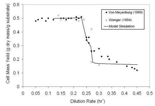
Figure 5. Chemostat or continuous culture steady state data on cell mass yield on glucose
The transition from the oxidative to fermentative pathways occurs either gradually or abruptly, depending on other culture conditions, such as oxygen supply rates, controlled mainly by impeller agitation rates, which are different in these experimental studies.
At the intermediate dilution rates, as the cells are changing from oxidative to
fermentative metabolism, yeast cells can exhibit spontaneous metabolic oscillations over a range of
operating conditions, such as the agitation rate or oxygen mass transfer rate. Several experimentalists have
documented these oscillations in aerobic continuous cultures of yeast on glucose. The figure from Porro et
al. (1988) shows the sustained oscillations in all the metabolite concentrations measured in the continuous
bioreactor. The top panel shows the online measurement trace of dissolved oxygen concentration in the culture
medium, which is most readily obtained. The subsequent panels show off-line  measurements of ethanol, glucose, intracellular storage
carbohydrates (trehalose and glycogen), medium pH, and cell number concentration (#/ml). These spontaneous
oscillations change in shape, period and amplitude as the bioreactor operating conditions of dilution rate and
agitation rate are varied within their oscillatory ranges. As these operating conditions are varied outside
their oscillatory range, the oscillations die down to either oxidative or fermentative consumption of
glucose.
measurements of ethanol, glucose, intracellular storage
carbohydrates (trehalose and glycogen), medium pH, and cell number concentration (#/ml). These spontaneous
oscillations change in shape, period and amplitude as the bioreactor operating conditions of dilution rate and
agitation rate are varied within their oscillatory ranges. As these operating conditions are varied outside
their oscillatory range, the oscillations die down to either oxidative or fermentative consumption of
glucose.
The metabolic oscillations can also be predicted by the yeast cybernetic model equations given above (Jones and Kompala, 1999) but requires the use of a stiff ODE solver. The simulations were conducted on the Berkeley Madonna software at the operating conditions of dilution rate of 0.16 hr-1 and oxygen mass transfer rate kLa (strongly affected by the agitation rate) of 300 hr-1. The parameter values for the different model constants are listed in the Table R.7.4.1.
At different operating conditions, the cybernetic model predicts also the experimentally observed trends in the shape and period of oscillations as well as the damping of the oscillations to either the fermentative or the oxidative consumption outside the range of oscillatory conditions.
POLYMATH TABLE:
Variable initial value minimal value maximal value final value
t 0 0 20 20
Cc 0.1 0.1 1801.2431 1801.2431
Cg 0.1 -1.115E+04 0.1 -1.115E+04
Ce 0.1 0.1 5328.5516 5328.5516
Co 1.2 0.0355565 1.2 0.0355565
e1 8.3E-05 8.3E-05 0.307713 0.3075931
e2 1.0E-04 1.0E-04 0.1591422 0.1034548
e3 1.0E-04 1.0E-04 0.1561239 0.0816329
Ct 0.1 2.022E-07 0.1 2.022E-07
beta1 0.7 0.7 0.7 0.7
gam3 0.8 0.8 0.8 0.8
mu1max 0.44 0.44 0.44 0.44
Ko2 0.01 0.01 0.01 0.01
beta2 0.7 0.7 0.7 0.7
beta3 0.7 0.7 0.7 0.7
mu2max 0.19 0.19 0.19 0.19
mu3max 0.36 0.36 0.36 0.36
alpha3 0.3 0.3 0.3 0.3
Ko3 2.2 2.2 2.2 2.2
alpha1 0.3 0.3 0.3 0.3
alpha2 0.3 0.3 0.3 0.3
e3max 0.2830189 0.2830189 0.2830189 0.2830189
e1max 0.2631579 0.2631579 0.2631579 0.2631579
e2max 0.3370787 0.3370787 0.3370787 0.3370787
E3 3.533E-04 3.533E-04 0.5500233 0.2884363
E1 3.154E-04 3.154E-04 1.1693077 1.1688539
E2 2.967E-04 2.967E-04 0.4714474 0.306916
K1 0.05 0.05 0.05 0.05
K2 0.01 0.01 0.01 0.01
K3 0.001 0.001 0.001 0.001
mu1 9.252E-05 -0.0902675 0.5389082 0.514298
mu2 5.082E-05 5.082E-05 0.0759984 0.0455136
mu3 4.445E-05 -0.096317 0.1036095 -7.893E-04
mumax 9.252E-05 9.252E-05 0.5389082 0.514298
u1 0.4926746 0.1706477 0.9199956 0.9199956
u2 0.2706217 -0.5804814 0.3786179 0.0814164
Y1 0.16 0.16 0.16 0.16
Y2 0.75 0.75 0.75 0.75
Y3 0.6 0.6 0.6 0.6
u3 0.2367037 -0.0191929 0.8158622 -0.001412
alphastar 0.1 0.1 0.1 0.1
Cg0 10 10 10 10
Cs20 20 20 20 20
D 0 0 0 0
v3 0.4804464 -1.4054924 1 -0.0015348
v1 1 -1.3172158 1 1
v2 0.5492909 0.0884965 1 0.0884965
sigmamuv 1.418E-04 1.418E-04 0.5457286 0.518327
dCc 1.418E-05 1.418E-05 933.63294 933.63294
gam1 10 10 10 10
gam2 10 10 10 10
dCt -1.175E-04 -0.0877451 0.062198 -1.838E-07
phi1 0.48 0.48 0.48 0.48
phi2 2 2 2 2
phi3 1 1 1 1
phi4 0.95 0.95 0.95 0.95
kla 300 300 300 300
Costar 0.1 0.1 0.1 0.1
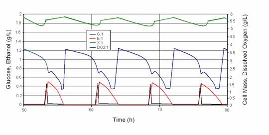
Figure 7. Cybernetic model simulations of metabolic oscillations in yeast continuous cultures. The shape and period of the oscillations in all the metabolite concentrations agree qualitatively with the experimental data. As the bioreactor operating conditions of D and kLa are changed, the shape and period of oscillations change as well in both experimental data and model simulations.
|
Parameter |
Units |
Definition |
Value |
|
|
mmax,1 |
hr-1 |
Max. Specific Growth Rate for Glucose Fermentation |
0.44 |
|
|
mmax,2 |
hr-1 |
Maximum Specific Growth Rate for Ethanol Oxidation |
0.19 |
|
|
mmax,3 |
hr-1 |
Maximum Specific Growth Rate for Glucose Oxidation |
0.36 |
|
|
K1 |
g/L |
Monod Saturation Constant for Glucose Fermentation |
0.05 |
|
|
K2 |
g/L |
Monod Saturation Constant for Ethanol Oxidation |
0.01 |
|
|
K3 |
g/L |
Monod Saturation Constant for Glucose Oxidation |
0.001 |
|
|
KO2 |
g/L |
Oxygen Saturation Constant for Ethanol Oxidation |
0.01 |
|
|
KO3 |
g/L |
Oxygen Saturation Constant for Glucose Oxidation |
2.2 |
|
|
Y1 |
g/g |
Yield Coefficient for Glucose Fermentation |
0.16 |
|
|
Y2 |
g/g |
Yield Coefficient for Ethanol Oxidation |
0.75 |
|
|
Y3 |
g/g |
Yield Coefficient for Glucose Oxidation |
0.60 |
|
|
ai |
hr-1 |
Enzyme Synthesis Rate Constant |
0.3 |
|
|
a*i |
hr-1 |
Constitutive Enzyme Synthesis Rate Constant |
0.1 |
|
|
bi |
hr-1 |
Enzyme Degradation Rate Constant |
0.7 |
|
|
g1 |
g/g |
Rate Constant for Carbohydrate Degradation |
10 |
|
|
g2 |
g/g |
Rate Constant for Carbohydrate Degradation |
10 |
|
|
g3 |
g/g |
Rate Constant for Carbohydrate Synthesis |
0.8 |
|
|
f1 |
g/g |
Stoichiometric Coefficient for Ethanol Production |
0.48 |
|
|
f2 |
g/g |
Stoichiometric Coefficient for Ethanol Oxidation |
2 |
|
|
f3 |
g/g |
Stoichiometric Coefficient for Glucose Oxidation |
1 |
|
|
f4 |
g/g |
Stoichiometric Coefficient for Carbohydrate Production |
0.95 |
|
|
CG,0, CS0, |
g/L |
Inlet or Feed Glucose and Substrate Concentrations |
10, var. |
|
|
CC |
g/L |
Cellmass Concentration |
variable |
|
|
CS, CS1, CS2 |
g/L |
Substrate Concentration |
variable |
|
|
CG, CE,, CO |
g/L |
Glucose, Ethanol, and Dissolved Oxygen concentrations |
variable |
|
|
CT |
g/g |
Intracellular Storage Carbohydrate (Trehalose) Conc. |
variable |
|
|
eI, emax,i |
g/g |
Intracellular Enzyme Concentration and its maximum |
variable |
|
|
Ei |
- |
Relative Amount of Intracellular Enzyme |
variable |
|
|
mi |
hr 1 |
Growth Rate on i'th Substrate or Pathway |
variable |
|
|
D |
hr 1 |
Dilution Rate |
variable |
|
|
u |
- |
Cybernetic Variables Controlling Enzyme Synthesis |
variable |
|
|
v |
- |
Cybernetic Variables Controlling Enzyme Activity |
variable |
|
|
kLa |
hr 1 |
Mass transfer coefficient for Dissolved Oxygen |
variable |
|
1. Kompala, D.S., D. Ramkrishna, N.B. Jansen and G.T. Tsao, "Investigation of bacterial growth on mixed substrates. Experimental evaluation of cybernetic models," Biotechnology and Bioengineering 28:1044-1055 (1986).
2. Jones, K.D. and D.S. Kompala, "Cybernetic model of the growth dynamics of Saccharomyces cerevisiae in batch and continuous cultures," J. Biotechnology 71: 105-131 (1999).
1. Show that the enzyme modification of the Monod growth kinetics is capable of simulating the presence or absence of the initial lag phase by varying the initial level of the intracellular enzyme content.
2. Show that the enzyme modification of Monod growth kinetics does not affect the chemostat profiles of cell mass and substrate over the range of dilution rates as well as the washout and optimal dilution rates.
3. Examine whether the order of substrate preference is affected by the choice of initial levels of the two key combinations (test the four combinations: high-high, high-low, low-high, and low-low where high represents 99% of emax,i and low represents 1% of emax,i).
4. Esherichia coli grows on a mixture of three sugars: glucose, xylose and lactose. The Monod growth rate parameters for glucose are: mmax,G = 1.2 hr-1, KG = 0.01 g/L, YC/G = 0.55 g/g; for xylose: mmax,X = 1.05 hr-1, KX = 0.05 g/L, YC/X = 0.52 g/g; and for lactose: mmax,L = 0.8 hr-1, KL = 0.1 g/L, YC/L = 0.45 g/g. How will these sugars be consumed in a batch bioreactor with the initial sugar concentrations of 5 g/L glucose, 10 g/L xylose, and 25 g/L of lactose. Extend the cybernetic model framework to address three substrates.
5. E. coli is to be cultured in a chemostat on a mixture of glucose, xylose and lactose with the feed concentrations of 5 g/L glucose, 10 g/L xylose, and 25 g/L of lactose. The Monod growth rate parameters are same as the ones in the problem above. What is the optimal dilution rate that will maximize the cell mass production rate (D*Cc)?
6. Zymomonas mobilis has been engineered to ferment pentoses like xylose in addition to the common hexose, glucose. The Monod parameters for this metabolically engineered microorganism during growth on glucose are mmax = 0.40 hr-1, Ks = 0.1 g/l, Yx/s = 0.11 gdw / gS, and Yp/s = 0.48 g ethanol / g glucose. The same parameters for growth on xylose are mmax = 0.30 hr-1, Ks = 0.5 g/l, Yx/s = 0.10 gdw/gS, and Yp/s = 0.45 g ethanol/g xylose. These cells are grown in a chemostat fermentor with the feed containing 50 g/l glucose and 50 g/l xylose. Using the Monod chemostat equations, calculate the maximum ethanol production rate possible from these cells growing in a chemostat. Assume that the fermentative growth on xylose gets repressed or shut off completely when the glucose concentration exceeds 0.2 g/l and that both sugars are fermented at lower dilution rates or glucose concentration < 0.2 g/l. Make any other assumptions as needed.
7. Solve the above problem using the cybernetic model equations, using a = 0.0001 and b = 0.05 for both key enzymes and without using the assumptions stated in the last two sentences of above problem.
8. Continuing with the theme of above problem, a second chemostat (of the same size) is added in series or downstream from the first chemostat, operated at high dilution rate, to ensure that all of xylose is consumed in continuous culture,. What dilution rate should be used to maximize the ethanol production rate from the metabolically engineering Zymomonas mobilis? Use the growth parameters from the earlier problem statement. Use the cybernetic model equations or state your additional assumptions.
9. Saccharomyces cerevisiae grows in a typical diauxic growth phenomenon on a mixture of glucose and galactose. The Monod growth rate parameters for the fermentative growth on galactose are assumed to be mmax = 0.40 hr-1, Ks = 0.1 g/L, Yx/s = 0.15 g cell mass / g galactose, and Yp/s = 0.47 g ethanol / g galactose. The growth rate parameters for oxidative growth on galactose are assumed to be mmax = 0.33 hr-1, Ks = 0.001 g/L, KO3 = 2.5 g/L and Yx/s = 0.58 g cell mass / g galactose. Similar parameters for growth on glucose and ethanol are given in Table R.7.4.1. Determine how the cell mass, glucose, galactose and ethanol profiles will be in batch culture on a mixture of 10 g/L glucose and 20 g/L galactose, if the inoculum is taken from continuous cultures on a mixture of glucose and galactose at a dilution rate.
10. Continuing with the theme of the above problem, S. cerevisiae is grown in a chemostat on a mixture of glucose and galactose, with the feed concentration of each being 50 g/L. It is desired to maximize the cell mass production rate (D*Cc). What should be the dilution rate used in the single chemostat, assuming a kLa of 1000 hr-1? Watch out for the possibility of spontaneous metabolic oscillations.
11. Continuing with the theme of the above problem further, S. cerevisiae is grown in a chemostat on a mixture of glucose and galactose, with the feed concentration of each being 50 g/L, to maximize the ethanol production rate (D*CE). What should be the dilution rate used in the single chemostat, assuming a kLa of 100 hr-1?
12. Simulate the metabolic oscillations of yeast, using the cybernetic model parameters in Jones and Kompala (1999) (given in the Table R.7.4.1) to (a) Plot how the period of oscillations changes with dilution rate D and (b) Plot how the period changes with the mass transfer coefficient, kLa. Use a stiff equation solver in your simulations to obtain the oscillations.
13. It has been found experimentally that the spontaneous metabolic oscillations in continuous cultures of yeast S. cerevisiae can be avoided by adding a small amount of ethanol to the feed stream, along with glucose feed concentration of 30 g/L. Investigate whether the cybernetic model equations given in section R.7.4.4 can predict the elimination of oscillations with the inclusion of ethanol in the feed stream. What is the smallest ethanol concentration that will eliminate the oscillations?
14. Determine the parameter sensitivity of the cybernetic model simulations of spontaneous metabolic oscillations in continuous cultures of yeast for the following assumed parameter values: a, a*, b, mmax,3, K3, KO3 and Y3. First obtain the oscillations through numerical simulations of the cybernetic model for any combination of bioreactor operating parameters, D and kLa. Next vary each of the assumed parameters to determine if and how the shape and period of oscillations change from the base case.
1) Introduction
In this laboratory exercise, we will study the growth characteristics of the yeast Saccharomyces cerevisiae in batch cultures. A lab-scale (5 liter) fermentor will be used to study batch growth kinetics of the yeast growing on glucose as the single carbon substrate provided in the presence of oxygen. A second fermentor will also contain glucose as the sole carbon substrate for the yeast to utilize in the absence of oxygen. A third lab-scale fermentor will be used to observe the growth behavior when the cells are presented with a mixture of two carbohydrates, glucose and glycerol in the presence of oxygen. You will take samples from the fermentors, measure the cell mass concentration (through optical density) and determine the concentrations of glucose and ethanol with spectrophotometric assay kits. With the accumulated results from the all the students over eighteen hours for the three different fermentors, you will be able to analyze the kinetics of cell growth, and the different patterns of multiple substrate utilization in batch cultures.
Yeast Metabolism
Saccharomyces cerevisiae uses the following three major pathways for growth on glucose:
1) The fermentation of glucose, which occurs primarily when the glucose concentration is high or when oxygen is not available. The cells attain a maximum specific growth rate of about 0.45 hr-1 with a low biomass yield of 0.15 g dry mass per gram glucose consumed and a high respiratory quotient (the ratio of CO2 production rate to the O2 consumption rate) and a low energy yield of only about 2 ATP per mole of glucose metabolized. The stoichiometry of this reaction is
C6H12O6 --------------> 2C2H5OH + 2CO2 + e
where e represents chemical energy utilized in the growth processes.
2) The oxidation of glucose, which predominates at glucose concentrations below 50 mg/l in aerobic cultures. The cells attain a maximum specific growth rate of only about 0.25 hr-1 with a biomass yield of about 0.5 g dry mass per gram glucose consumed, a respiratory quotient of about 1, and a high energy yield of 16-28 ATP per mole of glucose metabolized. The stoichiometry of this reaction is:
C6H12O6 + 6O2 --------------> 6CO2 + 6H2O + e
3)The oxidation of ethanol, which predominates when fermentative substrates are not available or in very limited supply. The cells attain a maximum specific growth rate of about 0.2 hr-1 with a high biomass yield of about 0.6-0.7 g dry mass per gram ethanol consumed, a low respiratory quotient of about 0.7, and an energy yield of about 6-11 ATP per mole of ethanol metabolized. The stoichiometry of this reaction is:
C2H5OH + 3O2 --------------> 2CO2 + 3H2O + e
Utilization of glycerol (the second carbon substrate provided in the third fermentor) by Saccharomyces cerevisiae is repressed by glucose. After the depletion of the faster growth-supporting substrate, glucose, the enzymes necessary for the assimilation of glycerol is induced, and an exponential growth phase on glycerol is expected to follow a diauxic lag phase.
Experimental Conditions
The temperature of the water bath surrounding the fermentors will be controlled at 30˚C, and the impellers inside each fermentor will be operated at 400 rpm. Two of the three fermentors will have glucose as the only initial carbon source at a concentration of 10 g/l. The other batch fermentor will have two initial carbon sources - glucose at 3 g/l and glycerol at 7 g/l. Air will be sparged into the first and the third fermentors at constant rate of 10 l/min. The dissolved oxygen concentration in all the three fermentors can be computer controlled to maintain a desired level by enriching the oxygen concentration in the sparged gas.
Introduction to Lab Procedures
You will monitor the growth characteristics of the yeast in the batch fermentors in three ways - by measuring the concentration of cells, and preparing cell-free samples at hourly intervals from each bioreactor for assaying the concentrations of glucose and ethanol. Yeast cell concentration can be determined indirectly by measuring the optical density (absorbance) of a culture sample. You will take a sample of the culture medium from the fermentor and read its absorbance using a spectrophotometer. Up to a certain cell density, the concentration of yeast cells (gdw/l) in the sample is proportional to the absorbance reading on the spectrophotometer. The calibration curve correlating cell concentration with absorbance deviates from a linear correlation at high cell densities. Because of this, it's a good idea to dilute any of your high OD samples (that may be on the non-linear portion of the curve) by a known dilution factor to confirm that the measured OD values fall on the linear portion.
The concentration of glucose, (glycerol) and ethanol in the cell-free culture samples will be analyzed by high performance liquid chromatography or spectrophotometric assay. To remove the cells from a 3 ml sample, the cell suspension will be centrifuged and the supernatant will be filtered through a microfiltration syringe, and assayed for glucose and ethanol by the spectrophotometric assay.
2) Experimental Procedures
A) Determining Cell Concentration
1) Zeroing the spectrophotometer. Set the wavelength to 630 nm. Using the knob on the left, set the reading to 0% transmission when the chamber is empty; using the knob on the right, set the reading to 100% transmission when the chamber contains a test tube with about 4 ml of pure medium.
2) Determining cell concentration. First flush out the sample tube for your group's fermentor by taking an 8-10 ml sample, which you will then discard. Take another 8-10 ml sample from your group's fermentor and gently mix. Take about 4 ml from your sample tube and transfer it to a glass test tube. Clean the outside of the test tube with ethanol, insert it into the spectrophotometer, and record the absorbance reading. If the absorbance reading is greater than 0.25, a typical limit of linear correlation between the absorbance and cell mass concentration, dilute the sample with a known amount of pure medium, and measure the absorbance again to check if the absorbance reading is on the linear portion of the calibration curve. Record the time you take the sample along with the absorbance reading in the linear range as well as the dilution factor.
B) Spectrophotometric Assays for Glucose and Ethanol
To remove the cells from a 3 ml sample, the culture will be centrifuged and the supernatant will be filtered through a microfiltration syringe. The lab TA will provide more details on the assay procedures during the experiment.
3) Report - Due February 19, 1997
A) Draw a graph of:
a) Logarithm of cell concentration vs. time
b) Glucose concentration vs. time
c) Ethanol concentration vs. time
for each of the three batch fermentors.
B) Determine the specific growth rate and the yield coefficient (gram dry weight of cells produced per gram of carbon source consumed) for each growth phase in the three fermentors. (The calibration between the absorbance reading and the dry cell mass concentration of the yeast cells will be performed at the end of the batch cultures and provided in the following class period).
C) Interpret these two graphs in light of the background information on yeast metabolic pathways and the "cybernetic" principle that cells choose to grow at the fastest possible rate. Specifically, discuss why the cell mass, glucose, (glycerol) and ethanol concentration profiles look as they do for each batch fermentor.