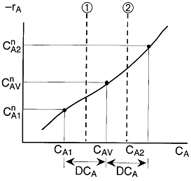
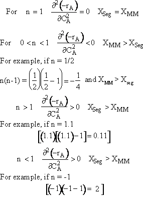
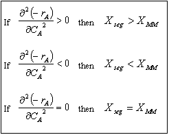
In the segregation model amd tje maximum mixedness model, one has to be able to perceive any macroelement of a fluid composed of numerous microelements. Macroelements have physical dimensions, but microelements don't have any physical dimension (like a point). When we consider mixing within a reactor with respect to the microelements present in the reactor, we can view two extreme levels of mixing. In one extreme, microelements are retained in a single macroelement. In other words, each macroelement is independent of another macroelement, and only the microelements within a macroelement mix with each other. This level of micromixing is called complete segregation. The other extreme level of micromixing is when microelements can permeate through the boundary of a macroelement. In other words, microelements from one macroelement can mix with microelements from another macroelement. In this type of mixing, all macroelements eventually loose their identity. This level is called maximum mixedness. Hence, we can see that in the segregation model, the different macroelements behave like batch reactors. In the maximum mixedness model, however, this is not the case because microelements of different macroelements can mix together.
We have considered two extreme levels of micromixing. As we discussed in the text, there are also two extreme levels of macromixing. At one extreme, we have an ideal PFR that has no macromixing; at the other extreme, we have a stirred tank that has a maximum degree of macromixing. For a better understanding of mixing in a reactor, let us consider Figure R13.3-1. As can be seen, in a stirred tank, micromixing can take place at any level. In other words, a stirred tank allows us to have both segregation (the point on the x-axis) and also maximum mixedness (the uppermost point on the vertical line). This point corresponds to an ideal CSTR. In other words, an ideal CSTR is a stirred tank having the maximum level of micromixing (i.e. maximum mixedness). As also can be seen, an ideal PFR is a reactor where both micromixing and macromixing are absent. In other words, one microelement does not mix with any other microelement in the PFR. In between an ideal PFR and an ideal CSTR, we can have different kinds of real reactors that can show both segregation and maximum mixedness. The level of micromixing, however, will be highest for an ideal CSTR and will decrease as we approach an ideal PFR.
R13.3.1 Segregation Model
For the two microelements (say 1 and 2) flowing together in the reactor, which may or may not be macroscopically well mixed, the segregation model can be pictured as shown in Figure R13.3-2.Here, there is no exchange of reactants among macroelements, but there is complete mixing of microelements in each macroelement. Hence, each macroelement can be visualized as a well-mixed batch reactor.
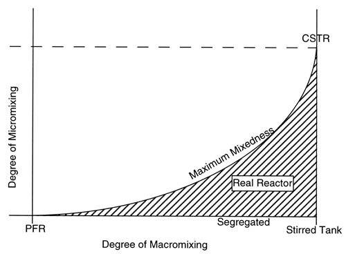
Figure R13.3-1
Mixing Extremes
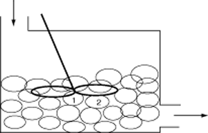
Segregation
R13.3.2 Maximum Mixedness Model
The maximum mixedness model can be visualized as shown in Figure R13.3-3.
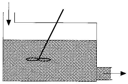
Figure R13.3-3
Micromixing
There is complete mixing and exchange of microelements among all macroelements.
Hence, the boundaries of all macroelements are not defined and we can
not distinguish one macroelement from another. The two macroelements,
1 and 2, (as shown in Figure R13.3-2 for the segregated model) are completely
mixed here. In the segregation model, these two macroelements have different
ages (i.e. different arriving time to the reactor), hence they have different
concentrations.
Let us assume that the reactant concentrations and volumes of these two
elements are CA1, CA2,
V1, and V2,
respectively.


 ĀĀĀĀĀĀĀĀĀĀĀĀĀ


 is
greater than


