Chapter 17: Distributions of Residence Times for Chemical Reactors
Self Test 17.7: Maximum Mixedness Model
Calculate the conversion predicted by the maximum mixedness model for a second order reaction in a reactor with the following RTD
E(t) = 0 for 0 < t 10s
E(t) = 0.01 (t–10) for 10 < t < 20
E(t) = 0.01 (30–t) for 20 < t < 30
E(t) = 0 for t > 30
The rate law is![]() with
with![]() and
and![]()


Solution
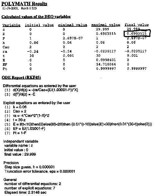
ODE Solver Solution
We will use the polymath solution rule than the graphical solution

The maximum time at which E(t) is not zero is 30 seconds. Therefore
Let z = 30 – l or l = 30 – z


![]()
![]()

The RTD function can be expressed as
![]()
However, remember E(t) = E(l)


Numerical Solution
|
l |
0 |
10 |
12 |
14 |
16 |
18 |
20 |
22 |
24 |
26 |
28 |
29 |
29.5 |
30 |
|
E(l) |
0 |
0 |
0.02 |
0.04 |
0.06 |
0.08 |
0.1 |
0.08 |
0.06 |
0.04 |
0.02 |
0.01 |
0.005 |
0 |
|
F(l) |
0 |
0 |
0.02 |
0.079 |
0.18 |
0.32 |
0.5 |
0.68 |
0.82 |
0.92 |
0.98 |
0.99 |
0.9986 |
0 |
|
EF=E(l) |
0 |
0 |
0.025 |
0.044 |
0.073 |
0.118 |
0.2 |
0.25 |
0.33 |
0.5 |
1.0 |
2.1 |
4.1 |
0 |
|
1–F(l) |
|
|
|
|
|
|
|
|
|
|
|
|
|
|
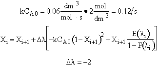
Calculate backwards starting at l = 30

l = 30 X = 0
l = 28 X = 0 + (–2) [–0.12 (1–0)2 + (0) (1.0)] = 0.24
l = 26 X = 0.24 + (–2) [–0.12 (1–0.24)2 + (0.24) (0.5)] = 0.14
l = 24 X = 0.14 + (–2) [–0.12 (1–0.14)2 + (0.14) (6.33)] = 0.22
l = 22 X = 0.22 + (–2) [–0.12 (1–0.22)2 + (0.22) (0.25)] = 0.26
l = 20 X = 0.26 + (–2) [–0.12 (1–0.26)2 + (0.26) (0.2)] = 0.287
l = 18 X = 0.341
l = 16 X = 0.395
l = 14 X = 0.45
l = 12 X = 0.45 + (–2) [–0.12 (1–0.45)2 + (0.45) (0.25)] = 0.5
l = 10 X = 0.5 + (–2) [–0.12 (1–0.5)2 + (0.5) (0)] = 0.56
l = 8 X = 0.56 + (–2) [–0.12 (1–0.56)2 + (0.56) (0)] = 0.666
l = 6 X = 0.643
l = 4 X = 0.678
l = 2 X = 0.7
l = 0 X = 0.72
One notes a slight difference between the conversion predicted by the software solution (X = 0.69) and that predicted by the backward integration using the very approximate Euler method. We would have achieved closer agreement if we had chosen a small step size, especially at the beginning.