WRFv4.0 Ideal Case - A Tropical Cyclone
当下需要使用WRF来进行既简单且理想情景的模拟,需要知道的是WRF在1, 2, 4, 8, 16, 32 core(s) 情形下的运算速度以及并行的线性性如何。
Run the case- A tropical cyclone
The case is WRF inbuilt ideal test, we are not required to use any real data, this greatly save our effect in preparing data using WPS.
According to the user guide in COMPILING WRF online tutorial, we change our present working directory to WRF/test/em_tropical_cyclone/.
The first thing we need to do is link the mandatory data to our PWD, literally by run the cshell script ./run_me_first.csh.
Here, we can slightly modifly its content so as to link the source as absolute paths, this is worthy of doing if you want to copy this test to elsewhere and keep the links as it is.
#!/bin/csh |
Then, we need to init the input files by run ./ideal.exe, which reads the namelist.input file and generates few outfiles: namelist.output, wrfinput_d01.
Then, we run WRF model by mpirun -np 8 wrf.exe, you may change the core number as you want to run the test concurrently, the model will evenly split the domain into several subblocks as you specified and distribute them to different cores.
All cores solely do the time ingeration, and they communicates for each step.
Finally, you may reach a completed result by finding a SUCCESS in you logfile.
The case itself
The test is set to be ideal case, with a default spatial extent of 200$\times$200, 20 vertical layers. dx=dy=15km, and dz=1.25km.
time duration is 6 days, the time step should assign to the 6$\times$dx = 90s. The output time interval I set is 60min, which means we get an ouput at each hour interval.
The result field as I simulated is shown here;
The case itself is modulated by the file: WRF/dyn_em/module_initialize_tropical_cyclone.f90, where inportant coefficients and inital conditions are defaultly specified, including:
- Initial State: The environment is horizontally homogeneous, with no initial wind (u = v = 0) and a static sea-surface temperature (SST) set at 28°C by default.
- Vortex: A weak, broad, axisymmetric vortex is added, balanced hydrostatically and in gradient-wind. Parameters for the vortex (such as r0, rmax, vmax, and zdd) can be modified in module_initialize_tropical_cyclone.F located in the dyn_em directory.
- Environment: An f-plane assumption holds, with the Coriolis parameter $f= 5.0\times 10^{-5}$, representing 20°N latitude.
- Boundary Conditions: Periodic lateral boundary conditions apply by default.
Computational efficiency
Simulations using different cores illuminate a computational efficiency curve: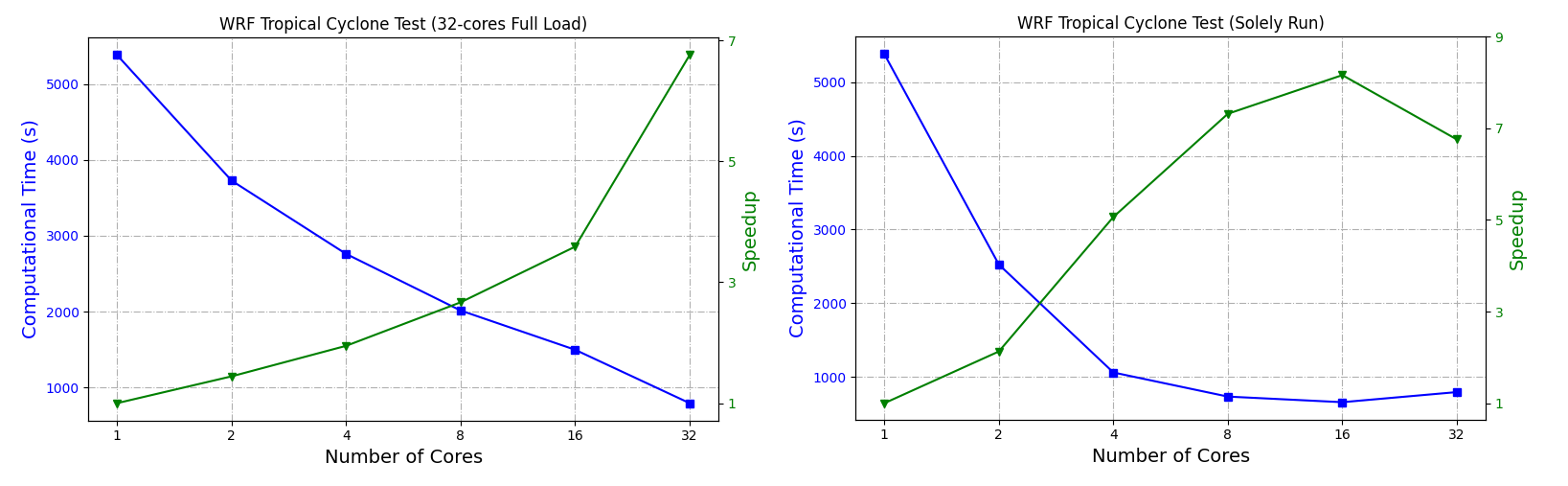
- The mpirun speedup is significant, while is limited by the I/O load, if all works submitted and run concurrently, the acceleration is remarkable.
- If the I/O is not busy, the speedup decays rapidly in this case. which means the acceleration is limited by the inter-blocks communications for such a small simulation.