Canoe Example#1：Straka Sinking Bubble

It has been 503 days since the last update, the content of the article may be outdated.

本节将通过一个具体的问题- Straka Problem的模拟来学习Canoe的编译和运行。
本模拟的模拟是通过考察高密度空气团的下沉和由此因此的边界层扰动，来评估模式在模拟刚性下表面情形的表现。空气的粘性流体，需要考虑由此引发的能量耗散。

问题描述

Strake Problem是Straka提出的，描述的是一个具有冷空气泡在二维大气中的下沉情形。其中大气是等熵的，水平范围是25.6 km,垂直6.4 km,两个维度的分辨率均为100 m，地表（1 bar）处的物理温度为 300K。

• 起始状态：
  空气泡的起始位置在（0, 3 km）处，气泡内部的温度分布遵循以下方程：
  $$\begin{array}{}\text{(1)}& \mathrm{\Delta }T=-15\text{K}\frac{\cos (\pi L)+1}{2},L<1\end{array}$$
  其中, L 为点 $(x,z)$ 到冷空气气泡中心点$(x_c,z_c)$的椭圆距：
  $$\begin{array}{}\text{(2)}& L=((\frac{x-x_c}{x_r}{)}^2+(\frac{z-z_c}{z_r}{)}^2{)}^{1/2}.\end{array}$$
  其中, $x_c=0$ km, $z_c=3$ km, $x_r=4$ km, $z_r=2$ km。

• 物理过程：
  起初，气泡处于流体静力稳定状态（hydrostatically balanced）；由于对流不稳定，气泡从起始位置开始下沉，并带动周围的空气流动，由此产生的密度流在界面上传播，形成Kelvin-Helmholtz不稳定。本example的目的就是对这一过程进行模拟。

模拟

$ cd 
$ mkdir -p StrakaProj/build
$ cd StrakaProj/build
$ cmake ~/canoe -DTASK=straka
$ make -j8
$ cd ..
$ln -s build/bin/straka.release .
$ ln -s build/bin/straka.release .
$ ln -s build/bin/combine.py .
$ cp build/bin/straka.inp .
$ ./straka.release -i straka.inp 
$ python combine.py -o test

实验进行了900s的模拟，生成了straka-test-main.nc文件，头信息：straka-test-main.headinfo。
脚本：make_plots.py。
绘制0，300，600，900s四个时刻的位温场的模拟：

python3 make_plots.py

2d.straka-theta(点击查看大图)

源码解析

源码位置不在本编译目录下，在canoe安装目录下：~canoe/examples/2019-Li-snap/straka.cpp
我们来逐行分析：

头文件

这里简单提一下，Athena++是原子物理层面，适用于量子力学/流体力学的天文磁流体模式。Canoe是在其基础内核上开发的，基于其网格并行架构(mesh,meshblock)、流体力学模块(hydro)和类的封装风格（airparcel）、重力（gravity），坐标（coordinate）, I/O等，加入了热力学模块（thermodynmics），辐射传输（radiation, opacity）等分子层面的宏观物理方法的大气模式。所以，canoe需要include很多athena++的类库，同时，自身要实现从atom到particle的转变。

#include <athena/athena.hpp>
#include <athena/athena_arrays.hpp>
#include <athena/stride_iterator.hpp>
#include <athena/parameter_input.hpp>
#include <athena/coordinates/coordinates.hpp>
#include <athena/eos/eos.hpp>
#include <athena/hydro/hydro.hpp>
#include <athena/field/field.hpp>
#include <athena/mesh/mesh.hpp>
#include <impl.hpp>
#include <snap/thermodynamics/thermodynamics.hpp>
#include <climath/core.h>

• athena.hpp：定义了Athena++的各种各种变量、类型、常量、下标，指针，结构体等等。 如：Real型，ConsIndex,PrimIndex等枚举类；

• parameter_input.hpp：设定了用于读取、存储模式输入文件<straka.inp>中变量的ParameterInput类型和GetInteger()，GetReal()等函数；

• coordinates.hpp：定义，存储和计算坐标位置，网格距和几何特性（面积、体积、source term）的文件；

• eos.hpp ：定义用于计算状态方程（Equation of State）的数据和函数；

• hydro.hpp ：这位更是重量级，定义了处理流体力学过程的Hydro类，负责处理流体动力过程中压强、密度和速度场的演变。包含了指向特定meshblock的指针*pmb; Hydro类本身可以被指针*hydro引用；Athena++还可以用来模拟磁流体力学过程 magnetohydrodynamics (MHD);

• field.hpp：负责处理磁流体力学中的场的变化，大气模拟一般用不到；

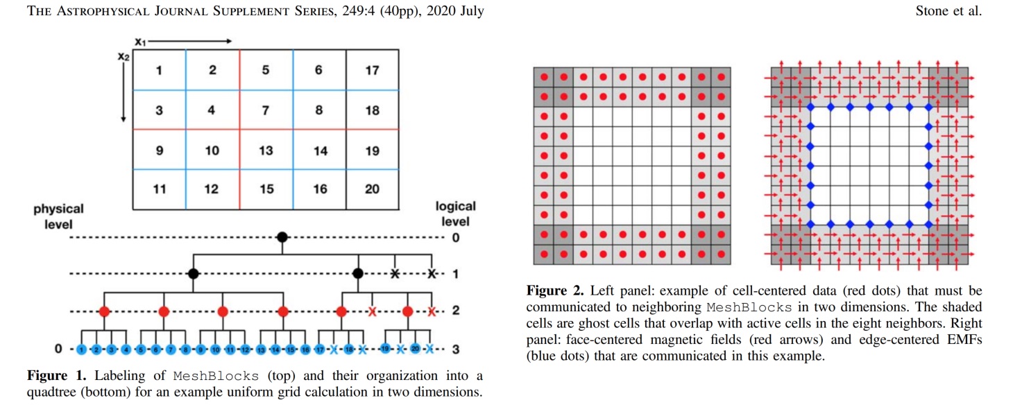
• mesh.hpp ：负责处理mesh和meshblock的类库，并且协调不同处理器并行情形下的mesh分布式计算问题。

  • MeshBlock class:格点类，控制单个格点的各种过程和位置信息；
  • Mesh class:所有网格类型的总类，结构上是由大量meshBlock示例构成；类别上可以分成规则网格，三角形网格、变分网格等。
  • Mesh网格的设计：参考Athena++团队发表的网格设计和工作原理：【The Athena++ Adaptive Mesh Refinement Framework: Design and Magnetohydrodynamic Solvers】;
    
    Mesh网格结构示意图
    
    详细内容会在mesh网格文章中介绍。（挖坑~）

• impl.hpp ：这是Canoe作为athena++扩展时为了灵活添加需要的物理方案和模块，留下的伪类，称为Opaque pointer，也可以理解为一个接口或后门，后续需要做任何模块的修改，只要子imp类中做扩展并具体实现就可以了。目前，impl类上插了以下几个canoe的实际物理/化学/辐射模块：radiation（辐射传输）,inversion（反演）,decomposition（分解）,thermodynamics（热力学）,turbulence_model（湍流）,microphysics（微物理）,chemistry（化学）,tracer（痕量气体）。

• MeshBlock类：这里介绍以下MeshBlock类，被定义在Mesh类的里面，负责管理每个格点的坐标、状态和相关物理过程的实现，在逻辑上后于Mesh类的实例化。这些物理是由其内部封装的指针来访问的，包括：

  • Coordinates *pcoord // 格点的坐标系统
  • Hydro *phydro // 流体力学过程
  • EquationOfState *peos // 大气状态方程
  • 但是，如*pthermo,*prad等属于Canoe扩展的类的指针，定义在impl高级包装类中。因为不属于MeshBlock类的成员指针，不能在其实例中直接使用，需要先实例化：auto pthermo = Thermodynamics::GetInstance();，或者通过impl类的指针来访问:auto prad = pimpl->prad;。

• thermodynamics.hpp ：定义在impl类中，负责处理热力学相关的过程和状态的解算。包含了温度、压强、位温、能量等参数的求算，以及：

  • 几种大气层结假设：

    enum class Method {
    ReversibleAdiabat = 0, // 可逆绝热
    PseudoAdiabat = 1, //假绝热
    DryAdiabat = 2, //干绝热
    Isothermal = 3, // 等温大气
    NeutralStability = 4 // 中性稳定
    };

  • 大气结构构建函数：

    //! Construct an 1d atmosphere
    //! \param[in,out] qfrac mole fraction representation of air parcel
    //! \param[in] dzORdlnp vertical grid spacing
    //! \param[in] method choose from [reversible, pseudo, dry, isothermal]
    //! \param[in] grav gravitational acceleration
    //! \param[in] userp user parameter to adjust the temperature gradient
    void Thermodynamics::Extrapolate(AirParcel* qfrac, Real dzORdlnp, Method method,
                                 Real grav, Real userp) const {
    qfrac->ToMoleFraction();
    
    // equilibrate vapor with clouds
    for (int i = 1; i <= NVAPOR; ++i) {
        auto rates = TryEquilibriumTP_VaporCloud(*qfrac, i);
    
        // vapor condensation rate
        qfrac->w[i] += rates[0];
    
        // cloud concentration rates
        for (int j = 1; j < rates.size(); ++j)
        qfrac->c[cloud_index_set_[i][j - 1]] += rates[j];
    }
    
    // RK4 integration
    #ifdef HYDROSTATIC
    rk4IntegrateLnp(qfrac, dzORdlnp, method, userp);
    #else
    rk4IntegrateZ(qfrac, dzORdlnp, method, grav, userp);
    #endif
    }

    这部分内容会在模式的大气热力学基础中讲（又挖坑~~~）

---

输出设置

接下来，程序定义了几个全局变量。这里，K 是运动粘度，p0是表面压力，cp 是比热容，而Rd 是干燥空气的理想气体常数。这里的普朗特数 是1。

Real K, p0, cp, Rd;

---

设置输出量：你在inp文件中看到的UOV就是这里的UserOutputVariable的缩写。这里输出了温度场和位温场作为诊断量。
为输出量分配内存：

void MeshBlock::InitUserMeshBlockData(ParameterInput *pin) {   
  AllocateUserOutputVariables(2);          // 声明两个输出量
  SetUserOutputVariableName(0, "temp");    // 命名
  SetUserOutputVariableName(1, "theta");
}

由于温度和位温仅用于输出目的，它们不需要在每个动态时间步长中计算。下面的子例程循环遍历所有网格，并在输出时间步长之前计算温度和位温的值。特别地，指向Thermodynamics类的指针pthermo使用其自己的成员函数Thermodynamics::GetTemp和PotentialTemp来计算温度和位温。

void MeshBlock::UserWorkBeforeOutput(ParameterInput *pin) {
  auto pthermo = Thermodynamics::GetInstance();
  // 循环遍历网格。js、je、is、ie是MeshBlock类的成员，
  // 它们是表示每个维度中网格的起始索引和结束索引的整数值。
  int k = ks; //本个例是二维场的模拟，第三维k=ks=1
  for (int j = js; j <= je; ++j)
    for (int i = is; i <= ie; ++i) {
      // user_out_var存储实际数据。
      // phydro是指向Hydro类的指针，它具有成员w，该成员存储每个网格的密度、压力和速度。
      user_out_var(0, j, i) = pthermo->GetTemp(this, k, j, i);
      user_out_var(1, j, i) = pthermo->PotentialTemp(this, p0, k, j, i);
    }
}

*pthermo是一个高级管理类MeshBlock的成员。因此，在MeshBlock类的成员函数中，您可以直接使用它。实际上，所有物理模块都由MeshBlock管理。只要您有一个指向MeshBlock的指针，您就可以访问模拟中的所有物理模块。

---

Forcing function

本个例中，明确要求考虑，下沉的气泡受到重力以及粘性和热耗散的影响。重力的作用已经由程序的其他部分处理，我们只需要编写几行代码来实现耗散。第一步是定义一个函数，该函数以指向MeshBlock的指针作为参数，以便通过该指针访问所有物理量。这个函数的名称并不重要，可以是任何名字。但是参数的顺序和类型必须是
void AnyName(MeshBlock*，Real const，Real const，AthenaArray const&，AthenaArray const&，AthenaArray&)
它们被称为函数的签名。

void Diffusion(MeshBlock *pmb, Real const time, Real const dt,
               AthenaArray<Real> const &w, AthenaArray<Real> const &r,
               AthenaArray<Real> const &bcc, AthenaArray<Real> &u,
               AthenaArray<Real> &s) {
  // <code>pcoord</code> is a pointer to the Coordinates class and it is a
  // member of the MeshBlock class. We use the pointer to the MeshBlock class,
  // <code>pmb</code> to access <code>pcoord</code> and use its member function
  // to get the spacing of the grid.
  Real dx = pmb->pcoord->dx1f(pmb->is);
  Real dy = pmb->pcoord->dx2f(pmb->js);

  // Similarly, we use <code>pmb</code> to find the pointer to the
  // Thermodynamics class, <code>pthermo</code>.
  auto pthermo = Thermodynamics::GetInstance();

  // Loop over the grids.
  int k = pmb->ks;
  for (int j = pmb->js; j <= pmb->je; ++j)
    for (int i = pmb->is; i <= pmb->ie; ++i) {
      // Similar to what we have done in MeshBlock::UserWorkBeforeOutput, we use
      // the Thermodynamics class to calculate temperature and potential
      // temperature.
      Real temp = pthermo->GetTemp(pmb, pmb->ks, j, i);
      Real theta = pthermo->PotentialTemp(pmb, p0, pmb->ks, j, i);

      // The thermal diffusion is applied to the potential temperature field,
      // which is not exactly correct. But this is the setting of the test
      // program.
      Real theta_ip1_j = pthermo->PotentialTemp(pmb, p0, k, j + 1, i);
      Real theta_im1_j = pthermo->PotentialTemp(pmb, p0, k, j - 1, i);
      Real theta_i_jp1 = pthermo->PotentialTemp(pmb, p0, k, j, i + 1);
      Real theta_i_jm1 = pthermo->PotentialTemp(pmb, p0, k, j, i - 1);

      u(IM1, j, i) += dt * K * w(IDN, j, i) / (dx * dy) *
                      (w(IVX, j, i - 1) + w(IVX, j, i + 1) + w(IVX, j - 1, i) +
                       w(IVX, j + 1, i) - 4. * w(IVX, j, i));
      u(IM2, j, i) += dt * K * w(IDN, j, i) / (dx * dy) *
                      (w(IVY, j, i - 1) + w(IVY, j, i + 1) + w(IVY, j - 1, i) +
                       w(IVY, j + 1, i) - 4. * w(IVY, j, i));

      // Adding thermal dissipation is similar to adding viscous dissipation.
      u(IEN, j, i) +=
          dt * K * w(IDN, j, i) / (dx * dy) * cp * temp / theta *
          (theta_ip1_j + theta_im1_j + theta_i_jp1 + theta_i_jm1 - 4. * theta);
    }
}

怎么理解这个Forcing function呢？Athena++的 hydro模块解决了一个流体力学的质量守恒和能量守恒问题。

首先，对与理想流体（粘性为0，受外力作用不发生粘性耗散），其满足的质量守恒方程（连续性方程）为：
$$\begin{array}{}\text{(3)}& \frac{\partial \rho }{\partial t}+▽\cdot (\rho u)=0;\end{array}$$

• $\rho$ is the density of the fluid.
• $u$ is the velocity of the fluid.
• $t$ is time.
  理解起来就是：局地变化项=平流项。

动量方程：

理想流体的动量方程是欧拉方程的一部分，描述了流体中动量的守恒。在一维流动中，动量方程可以写成：
$$\begin{array}{}\text{(4)}& \frac{\partial }{\partial t}(\rho u)+\frac{\partial }{\partial x}(\rho u^2+P)=0\end{array}$$

• $P$ is the pressure of the fluid.
• $x$ is the spatial coordinate.
• 这个方程表示了流体中动量的守恒。左侧第一项表示动量的时间变化率，第二项表示空间域中动量的平流通量。
  注：欧拉方程假设一个理想化的流体，没有粘性或热传导（无粘性和绝热）。在具有粘性和热效应的实际情况中，通常会使用包含粘性和热传导额外项的Navier-Stokes方程。

能量守恒方程：
理想流体的能量守恒方程可以通过欧拉方程来表示，该方程描述了无粘性和绝热的流体运动。欧拉方程包括连续性方程、动量方程和能量方程。

对于一维流动，理想流体的能量守恒方程可以写成：
$$\begin{array}{}\text{(5)}& \frac{\partial }{\partial t}(\rho E+\frac{1}{2}\rho u^2)+\frac{\partial }{\partial x}(\rho uE+\frac{1}{2}\rho u^3+Pu)=0\end{array}$$

• $E$ is the specific total energy, given by $E=e+\frac{1}{2}{u}^2$, where $e$ is the specific internal energy.
• 这个方程表示了流体中总能量（内能和动能）的守恒。它考虑了总能量的时间变化率以及在空间域内的能量通量。
  注：，欧拉方程假设了一个理想化的流体，没有粘性或热传导（无粘性和绝热）。在具有粘性和热效应的实际情况中，通常会使用包含粘性和热传导额外项的Navier-Stokes方程。

那么在Straka问题中，真实的大气是具有一定粘性的，受外力作用会发生热量耗散，方程就需要加上耗散项：

动量耗散项：
$$\begin{array}{}\text{(6)}& M_{\text{x}}(j,i)+=\frac{\partial t\cdot K}{\partial x\cdot \partial y}(u_{\text{x}}(j,i-1)+u_{\text{x}}(j,i+1)+u_{\text{x}}(j-1,i)+u_{\text{x}}(j+1,i)-4\cdot u_{\text{x}}(j,i))\end{array}$$
热耗散项：
$$\begin{array}{}\text{(7)}& E(j,i)+=\frac{\partial t\cdot K}{\partial x\cdot \partial y}\frac{c_p\cdot \text{T}}{\theta }({\theta }_{i+1,j}+{\theta }_{i-1,j}+{\theta }_{i,j+1}+{\theta }_{i,j-1}-4\cdot {\theta }_{i,j})\end{array}$$
其中 $M_x$表示$x$方向上的动量分量；$E$表示总能量，$u_x$为$x$方向的速度，$\theta$为位温，$T$为温度，$K$为粘度；

在添加了粘性耗散的Forcing之后，流体的运动方程就完整了，Hydro模块会结合重力场去求解流体的状态演变。

Primitive | Conserved
Forcing部分的代码中涉及了u，w两个范参数，分别代表了保守量和状态量，这是继承与Athena++的特征。
Athena++使用u来表示conserved variables，如density, momentums, total energy (kinetic + internal)。这些量是保守量，也是广延量，可扩展量； 而使用w来并表示primitive variables，如temperature, velocities, and pressure，这些量都是强度量，也是状态量。这两者在<AthenaArray.hpp>类库中定义：AthenaArray<Real> u, w

这一问题的说明请见【Appendix B: Conversion between Primitive Variables and Conserved Variables】

athena/src/athena.hpp 里这样定义这些变量的枚举下标：

//! array indices for conserved u : density, momemtum, total energy
enum ConsIndex {IDN=0, IM1=1, IM2=2, IM3=3, IEN=4};
//! array indices for face-centered field
enum MagneticIndex {IB1=0, IB2=1, IB3=2};

//! array indices for 1D primitives w: velocity, transverse components of field
enum PrimIndex {IVX=1, IVY=2, IVZ=3, IPR=4, IBY=(NHYDRO), IBZ=((NHYDRO)+1)};

//! array indices for face-centered electric fields returned by Riemann solver
enum ElectricIndex {X1E2=0, X1E3=1, X2E3=0, X2E1=1, X3E1=0, X3E2=1};

//! array indices for metric matrices in GR
enum MetricIndex {I00=0, I01=1, I02=2, I03=3, I11=4, I12=5, I13=6, I22=7, I23=8, I33=9,
                  NMETRIC=10};
//! array indices for triangular matrices in GR
enum TriangleIndex {T00=0, T10=1, T11=2, T20=3, T21=4, T22=5, T30=6, T31=7, T32=8, T33=9,
                    NTRIANGULAR=10};

由此，常用的一些量在程序中表示为：

w[IPR] = Press;
w[IDN] = Temperature;
w[IVX] = verlocity in dimension x
u[IDN] = Density
u[IM1] = Momentums in dimension x
u[IEN] = Total Energy

初始化Mesh类参数

这是初始化程序特定变量的地方。注意这个函数是Mesh类的成员函数，而不是我们一直在使用的MeshBlock类的成员函数。
Mesh类是一个全包括的类，管理多个MeshBlock，而MeshBlock类管理所有物理相关模块；在实例化这两个类的过程中，应该首先实例化Mesh类，然后它在内部实例化所有的MeshBlock。
因此，这个子程序在所有MeshBlock之前运行。

void Mesh::InitUserMeshData(ParameterInput *pin) {
  // 在这里设置程序特定的驱动参数。
  // 这些参数来自输入文件，由ParameterInput类解析。
  Real gamma = pin->GetReal("hydro", "gamma");  // gamma = C_p/C_v   specific heats
  K = pin->GetReal("problem", "K");    // viscious coefficient
  p0 = pin->GetReal("problem", "p0");  //  surface pressure
  Rd = pin->GetReal("thermodynamics", "Rd");  // specific gas constant for dry air [J/(kg·K)]
  cp = gamma / (gamma - 1.) * Rd;   // specific heat at constant pressure [J/(kg·K)]

  // 这行代码注册我们在上一部分中编写的Forcing Function。
  EnrollUserExplicitSourceFunction(Diffusion);
}

上述的，$K,P_0,R_d,c_p,\gamma$ 等参数都属于Mesh类的成员参数，适用于所有MeshBlock实例，而且此处要注册一个forcingfunction，所以要在此处先读取并Initalize。

初始化MeshBlock参数

这是程序的最后一部分，我们在其中设置初始条件。在Athena++应用程序中，一般称为problem generator。
这部分可以理解成初始时刻，对每个MeshBlock进行设置。

void MeshBlock::ProblemGenerator(ParameterInput *pin) {
  // 获取重力的值。正值表示向上，负值表示向下。
  // 我们取负值以获得绝对值。
  Real grav = -phydro->hsrc.GetG1();
  // 这些行读取输入文件中的参数值，这些参数以节的形式组织。
  // 问题特定的参数通常放在`<problem>`节下。
  Real Ts = pin->GetReal("problem", "Ts");
  Real xc = pin->GetReal("problem", "xc");
  Real xr = pin->GetReal("problem", "xr");
  Real zc = pin->GetReal("problem", "zc");
  Real zr = pin->GetReal("problem", "zr");
  Real dT = pin->GetReal("problem", "dT");

循环遍历网格。目的是在每个单元格中心网格上设置温度、压力和密度场。
按照straka problem的情景，初始时刻应该是：
1）有一个绝热大气的温压场，使用了大气状态方程（EOS, Equation of State）先对大气进行构建；
$$\begin{array}{}\text{(8)}& p=p_0(\frac{T}{T_s}{)}^{c_p/R_d}\end{array}$$
2）在此基础上叠加一个冷的气泡的温度异常导致的温度场，公式（1）。

for (int j = js; j <= je; ++j) {
  for (int i = is; i <= ie; ++i) {
    // 获取垂直和水平方向的笛卡尔坐标。`x1`通常是垂直方向，`x2`是水平方向。
    // `x1v`和`x2v`检索单元格中心的坐标。
    Real x1 = pcoord->x1v(i);
    Real x2 = pcoord->x2v(j);
    // 到（xc，zc）处冷空气泡中心的距离。
    Real L = sqrt(sqr((x2 - xc) / xr) + sqr((x1 - zc) / zr));
    // 绝热温度梯度。
    Real temp = Ts - grav * x1 / cp;
    // 一旦知道温度，就可以计算绝热和静力压力，公式为
    // $p=p_0(\frac{T}{T_s})^{c_p/R_d}$，其中$p_0$是地表压力，$T_s$是地表温度。
    phydro->w(IPR, j, i) = p0 * pow(temp / Ts, cp / Rd);
    if (L <= 1.) temp += dT * (cos(M_PI * L) + 1.) / 2.;
    // 使用理想气体定律设置密度。
    phydro->w(IDN, j, i) = phydro->w(IPR, j, i) / (Rd * temp);
    // 将速度初始化为零。
    phydro->w(IVX, j, i) = phydro->w(IVY, j, i) = 0.;
  }
}

我们已经设置了所有的primitive variables。最后一步是基于primitive variables计算conserved variables。
这是通过调用成员函数EquationOfState::PrimitiveToConserved完成的。
注意，pfield->bcc是一个占位符，因为这个示例中没有MHD涉及。

  peos->PrimitiveToConserved(phydro->w, pfield->bcc, phydro->u, pcoord, is, ie, js, je, ks, ke);
}

源码和输入文件

/* -------------------------------------------------------------------------------------
 * SNAP Example Program
 *
 * Contributer:
 * Cheng Li, University of Michigan
 *
 * Year: 2021
 * Contact: chengcli@umich.edu
 * Reference: Straka et al., 1993
 * -------------------------------------------------------------------------------------
 */
 
#include <athena/athena.hpp>
#include <athena/athena_arrays.hpp>
#include <athena/stride_iterator.hpp>
#include <athena/parameter_input.hpp>
#include <athena/coordinates/coordinates.hpp>
#include <athena/eos/eos.hpp>
#include <athena/hydro/hydro.hpp>
#include <athena/field/field.hpp>
#include <athena/mesh/mesh.hpp>
 
#include <impl.hpp>
 
#include <snap/thermodynamics/thermodynamics.hpp>
 
#include <climath/core.h>
 
Real K, p0, cp, Rd;
 
 
void MeshBlock::InitUserMeshBlockData(ParameterInput *pin) {
  AllocateUserOutputVariables(2);
  SetUserOutputVariableName(0, "temp");
  SetUserOutputVariableName(1, "theta");
}
 
void MeshBlock::UserWorkBeforeOutput(ParameterInput *pin) {
  auto pthermo = Thermodynamics::GetInstance();
 
  int k = ks;
  for (int j = js; j <= je; ++j)
    for (int i = is; i <= ie; ++i) {
      user_out_var(0, j, i) = pthermo->GetTemp(this, k, j, i);
      user_out_var(1, j, i) = pthermo->PotentialTemp(this, p0, k, j, i);
    }
}
 
 
void Diffusion(MeshBlock *pmb, Real const time, Real const dt,
               AthenaArray<Real> const &w, AthenaArray<Real> const &r,
               AthenaArray<Real> const &bcc, AthenaArray<Real> &u,
               AthenaArray<Real> &s) {
  Real dx = pmb->pcoord->dx1f(pmb->is);
  Real dy = pmb->pcoord->dx2f(pmb->js);
 
  auto pthermo = Thermodynamics::GetInstance();
 
  int k = pmb->ks;
  for (int j = pmb->js; j <= pmb->je; ++j)
    for (int i = pmb->is; i <= pmb->ie; ++i) {
      Real temp = pthermo->GetTemp(pmb, pmb->ks, j, i);
      Real theta = pthermo->PotentialTemp(pmb, p0, pmb->ks, j, i);
 
      Real theta_ip1_j = pthermo->PotentialTemp(pmb, p0, k, j + 1, i);
      Real theta_im1_j = pthermo->PotentialTemp(pmb, p0, k, j - 1, i);
      Real theta_i_jp1 = pthermo->PotentialTemp(pmb, p0, k, j, i + 1);
      Real theta_i_jm1 = pthermo->PotentialTemp(pmb, p0, k, j, i - 1);
 
      u(IM1, j, i) += dt * K * w(IDN, j, i) / (dx * dy) *
                      (w(IVX, j, i - 1) + w(IVX, j, i + 1) + w(IVX, j - 1, i) +
                       w(IVX, j + 1, i) - 4. * w(IVX, j, i));
      u(IM2, j, i) += dt * K * w(IDN, j, i) / (dx * dy) *
                      (w(IVY, j, i - 1) + w(IVY, j, i + 1) + w(IVY, j - 1, i) +
                       w(IVY, j + 1, i) - 4. * w(IVY, j, i));
 
      u(IEN, j, i) +=
          dt * K * w(IDN, j, i) / (dx * dy) * cp * temp / theta *
          (theta_ip1_j + theta_im1_j + theta_i_jp1 + theta_i_jm1 - 4. * theta);
    }
}
 
 
void Mesh::InitUserMeshData(ParameterInput *pin) {
  Real gamma = pin->GetReal("hydro", "gamma");
  K = pin->GetReal("problem", "K");
  p0 = pin->GetReal("problem", "p0");
  Rd = pin->GetReal("thermodynamics", "Rd");
  cp = gamma / (gamma - 1.) * Rd;
 
  EnrollUserExplicitSourceFunction(Diffusion);
}
 
 
void MeshBlock::ProblemGenerator(ParameterInput *pin) {
  Real grav = -phydro->hsrc.GetG1();
  Real Ts = pin->GetReal("problem", "Ts");
  Real xc = pin->GetReal("problem", "xc");
  Real xr = pin->GetReal("problem", "xr");
  Real zc = pin->GetReal("problem", "zc");
  Real zr = pin->GetReal("problem", "zr");
  Real dT = pin->GetReal("problem", "dT");
 
  for (int j = js; j <= je; ++j) {
    for (int i = is; i <= ie; ++i) {
      Real x1 = pcoord->x1v(i);
      Real x2 = pcoord->x2v(j);
      Real L = sqrt(sqr((x2 - xc) / xr) + sqr((x1 - zc) / zr));
      Real temp = Ts - grav * x1 / cp;
      phydro->w(IPR, j, i) = p0 * pow(temp / Ts, cp / Rd);
      if (L <= 1.) temp += dT * (cos(M_PI * L) + 1.) / 2.;
      phydro->w(IDN, j, i) = phydro->w(IPR, j, i) / (Rd * temp);
      phydro->w(IVX, j, i) = phydro->w(IVY, j, i) = 0.;
    }
  }
 
  peos->PrimitiveToConserved(phydro->w, pfield->bcc, phydro->u, pcoord, is, ie,
                             js, je, ks, ke);
}

#straks.inp
<comment>
sroblem   = Dense sinking bubble test
reference = Straka et al., 1993
configure = --prob=straka --nghost=3 -netcdf ## 不再使用这种方法

<job>
problem_id = straka       # problem ID: basename of output filenames

<output1>
file_type  = hst          # History data dump
dt         = 300.          # time increment between outputs

<output2>
file_type  = netcdf      # Binary data dump
variable   = prim         # variables to be output
dt         = 300.          # time increment between outputs

<output3>
file_type  = netcdf
variable   = uov
dt         = 300.

<time>
cfl_number = 0.9          # The Courant, Friedrichs, & Lewy (CFL) Number
nlim       = -1           # cycle limit
tlim       = 900          # time limit
xorder     = 5            # horizontal reconstruction order
integrator = rk3          # integration method
ncycle_out = 10           # output frequency

<mesh>
nx1        = 64           # Number of zones in X1-direction
x1min      = 0.           # minimum value of X1
x1max      = 6.4E3        # maximum value of X1
ix1_bc     = reflecting   # inner-X1 boundary flag
ox1_bc     = reflecting   # outer-X1 boundary flag

nx2        = 256          # Number of zones in X2-direction
x2min      = 0.           # minimum value of X2
x2max      = 25.6E3       # maximum value of X2
ix2_bc     = reflecting   # inner-X2 boundary flag
ox2_bc     = reflecting   # outer-X2 boundary flag

nx3        = 1            # Number of zones in X3-direction
x3min      = -0.5         # minimum value of X3
x3max      = 0.5          # maximum value of X3
ix3_bc     = periodic     # inner-X3 boundary flag
ox3_bc     = periodic     # outer-X3 boundary flag

<hydro>
grav_acc1   = -9.8
gamma       = 1.4         # gamma = C_p/C_v

<thermodynamics>
Rd          = 287.

<problem>
dT    = -15.
xc    = 0.
xr    = 4.E3
zc    = 3.E3
zr    = 2.E3
p0    = 1.E5
Ts    = 300.
K     = 75.

TODO LIST

• Athena++ Mesh网格介绍；
• 模式的大气热力学基础；
• 大气流体力学基础