晴空模拟流程

  • example_fwd例程
    /src/test/example_fwd.F90展示了对最通用简单的RTTOV晴空模拟案例,你只需要根据需求修改自己模拟输入即可。
    RTTOV模拟通常包含以下步骤,这也是本例程的结构。

    The usual steps to take when running RTTOV are as follows:

    1. Specify required RTTOV options
    2. Read coefficients
    3. Allocate RTTOV input and output structures
    4. Set up the chanprof array with the channels/profiles to simulate
    5. Read input profile(s)
    6. Set up surface emissivity and/or reflectance
    7. Call rttov_direct and store results
    8. Deallocate all structures and arrays

rttov coefficient输入字符串地址,例如可以输入54层FY3D MWRI应用先行数据集提供的coefficient参数表:
/home/hjh/rttov13/rtcoef_rttov13/rttov13pred54L/rtcoef_fy3_4_mwri.dat
rttov profile 输入,例程是按照格式化方式读入的,示例的廓线为:
/home/hjh/rttov13/rttov_test/test_example.1/prof.dat

  • 跳过文件中的注释行:CALL rttov_skipcommentline(iup, errorstatus)
  • 指定气体的单位:
    fortran
    ! 0 => ppmv over dry air
    ! 1 => kg/kg over moist air
    ! 2 => ppmv over moist air
    READ(iup,*) profiles(1) % gas_units
    profiles(:) % gas_units = profiles(1) % gas_units
    如果使用ERA5的水汽混合比Q,其单位是kg/kg,应当gas_units=1;
  • 随后依次是Pressure levels (hPa)Temperature profile (K)Water vapour profile (ppmv)的自上而下的51层廓线,Ozone profile (ppmv)的轮廓线没有考虑,在源码和廓线示例中都被注释了
  • 最下面是近地表和surface的参数,仪器参数,分别被读进profiles(iprof)%s2m; profiles(iprof)%skin; profiles(iprof)%elevation等结构中;
  • 这里还有一个simple cloud 参数,对于晴空,将cloud fraction设为0.0就可以忽略云的考虑:
    plaintext
    ! Cloud top pressure (hPa) and cloud fraction for simple cloud scheme
    500.00 0.0

个例实战(一) 理想晴空单柱正向模拟

设定:

  1. 使用参考大气廓线;
  2. 使用理想的地表发射率
  3. 只考虑水汽的吸收,不考虑O3、云等水凝物的吸收和散射

输入的设置如下:

fortran
example_fwd.F90
!========== Interactive inputs == start ==============
! coeff 文件
coef_filename='/home/hjh/rttov13/rtcoef_rttov13/rttov13pred54L/rtcoef_fy3_4_mwri.dat'
prof_filename='./prof.dat' ! 理想廓线
nprof=1 ! 单柱模拟
nlevels=51
dosolar=0 ! 不考虑日光
nchannels=10 ! 10个通道
channel_list=(/1,2,3,4,5,6,7,8,9,10/) ! 通道列表
nthreads=1 ! 单线程
bash
$ make -f Makefile_examples # 编译
$ ./example_fwd.exe ## 执行
path of coefficient file --------------
/home/hjh/rttov13/rtcoef_rttov13/rttov13pred54L/rtcoef_fy3_4_mwri.dat
path of file containing profile data ------------ ./prof.dat
number of profiles --------------- 1
number of profile levels ------------- 51
turn on solar simulations? (0=no, 1=yes) -------- 0
number of channels to simulate per profile ----------- 10
enter space-separated channel list ---------------
1 2 3 4 5 6 7 8 9 10
number of threads to use -------------------- 1

洋面模拟结果

这里是洋面的模拟结果(Surface type=1):

plaintext
CALCULATED BRIGHTNESS TEMPERATURES (K):
114.68 114.71 133.38 133.23 159.48 159.25 158.36 157.81 215.07 213.82

CALCULATED SURFACE TO SPACE TRANSMITTANCE:
0.9867 0.9867 0.9530 0.9530 0.8799 0.8799 0.9214 0.9214 0.7887 0.7887

CALCULATED SURFACE EMISSIVITIES:
0.379 0.379 0.408 0.407 0.427 0.426 0.472 0.470 0.606 0.599

这里可以看出,洋面的模拟emissivity在0.5以下,这是一个非常典型的洋面发射率值,并且随着频率升高,这是由Debye方程决定的,并且由于洋面的spacular特性,发射率存在极化差。
在如此低的背景输出情况下,模拟得到的天顶亮温在200K以下,对于晴空洋面,也较为合理。如果这时候出现云(240K以上),那么对比度会非常高,所以洋面云和降水反演算法的精度较高。

关于表面发射率的模拟
洋面的发射率模拟会考虑海温、盐度、洋面风速等物理量。一般来说,先计算海水的节点常数,随后进行Fresnel反射率计算,最后还要进行风速作用下的表面粗糙洋面的反射率修正。这个思想和陆面发射率模拟的思想是相通的,只不过陆面考虑的介质更复杂,表面的粗糙和风速也无关。所以,整个RTTOV模式只考虑了近地面风场,并且只有在进行洋面发射率模拟时才用到,在进行发射率反演及陆面模拟时,风速的输入是可选的。

陆面模拟结果

我们修改一下Surface type=0,可以进行陆面上空的辐射传输模拟。
输出结果如下:

plaintext
CALCULATED BRIGHTNESS TEMPERATURES (K):
256.79 256.79 253.56 253.56 256.05 256.05 252.24 252.24 261.27 261.27

CALCULATED SURFACE TO SPACE TRANSMITTANCE:
0.9867 0.9867 0.9530 0.9530 0.8799 0.8799 0.9214 0.9214 0.7887 0.7887

CALCULATED SURFACE EMISSIVITIES:
0.893 0.893 0.875 0.875 0.869 0.869 0.864 0.864 0.874 0.874

可以看出,RTTOV的MEM模块算出来的陆面emissivity在0.9左右,相应的TB模拟在250K以上,这个结果对于陆面理想模拟来说,较为合理。

自定义Emissivity

除了把Emissivity交给表面模块来计算,我们还可以手动设定输入,以服务于敏感性研究或变分反演方法:

fortran
...... 
! --------------------------------------------------------------------------
! 6. Specify surface emissivity and reflectance
! --------------------------------------------------------------------------
.......
! Calculate emissivity within RTTOV where the input emissivity value is
! zero or less (all channels in this case)
! 不进行地表发射率计算
calcemis(:) = .false.
! calcemis(:) = (emissivity(:) % emis_in <= 0._jprb)
! 为所有通道指定0.9的发射率
emissivity(:) % emis_in=0.9

输出的亮温模拟结果如下:

plaintext
CALCULATED BRIGHTNESS TEMPERATURES (K):
258.71 258.71 260.13 260.13 262.91 262.91 261.00 261.00 265.89 265.89

CALCULATED SURFACE TO SPACE TRANSMITTANCE:
0.9867 0.9867 0.9530 0.9530 0.8799 0.8799 0.9214 0.9214 0.7887 0.7887

CALCULATED SURFACE EMISSIVITIES:
0.900 0.900 0.900 0.900 0.900 0.900 0.900 0.900 0.900 0.900

这里可以看出,天顶亮温模拟的极化差为0,这是因为手动设定的Emissivity忽略了地表几何特征引起的反射率的极化差。而大气辐射传输则不会考虑偏振差异,因此有这样的结果;

除了以上方法,发射率还可以使用Emissivity Atlas作为输入,这个前面讲过,后面用到了会做相应介绍。

注意到上述三种情形:洋面、陆面和手动陆面情形下的大气透过率是一样的,也就是说,大气的辐射传输贡献和地表本身的辐射背景输入无关,基于这一原理,我们可以实现自上而下的反演计算。
辐射传输模式也表明了这一点:
$$
\begin{align}
Tb_{v,p}=T_u+Γ_v [e_{v,p} T_s+(1-e_{v,p}) T_d]
\\
e_{v,p}=(Tb_{v,p} - T_u - \tau_v T_d)/(τ_v (T_s-T_d))
\end{align}
$$

个例实战(二) 晴空轨道模拟

本个例将使用再分析资料进行2023.06.27日的FY上行轨道进行模拟, 模拟卫星观测到的轨道天顶亮温

试验设置

使用ERA5相关资料为RTTOV提供输入量,并使用风云的轨道经纬度信息模拟出卫星的实时观测。模拟设定如下:

  1. 不涉及像斑卷积和频率运算;
  2. 不考虑积雪、海冰和云的存在;
  3. 采用最邻近匹配廓线和地表近地表参数;
  4. 廓线取50GHz以下诸层,共29层;
  5. 2m比湿取廓线最底层的值;
  6. 洋面发射率和地表发射率交给模式模拟;
  7. 逐轨道模拟。

主要步骤:

  • 读取卫星Swath的观测几何参数
    fortran
    call read_FY_Vars(FY_FILENAME,nscan,npix,FYlon,FYlat,FYtbs,minsec,igbp,lsmask,dem,retcode)
    call read_FY_Geometry(FY_FILENAME,nscan,npix,sea,sez,soa,soz,retcode)
  • 匹配和下载ERA5资料
    fortran
    call system("python3 "//trim(adjustl(pwd))//"ERA5/era5-pl-download.py "//yyyymmdd//" "//UTC_str )	
    call system("python3 "//trim(adjustl(pwd))//"ERA5/era5-land-download.py "//yyyymmdd//" "//UTC_str )
    call system("python3 "//trim(adjustl(pwd))//"ERA5/era5-single-download.py "//yyyymmdd//" "//UTC_str )
  • 读取ERA5参数
    fortran
    call read_ERA5_profs(req_era5,lon,lat,qw,rh,ta,zg)
    call read_ERA5_surfs(req_surf,lst,psrf,t2m) !! K, hPa, K !! 1 (top) -> 29 (bottom)
    call read_ERA5_sigls(req_sigl,sst,psrf,t2m,u10,v10)
  • 调用RTTOV
    fortran
    call rttov_clearsky_fwd(npix,FYlon,FYlat,plevel,&
    qw,ta,skt,psrf,t2m,u10,v10,dem,lsmask,sea,sez,soa,soz,simu)
  • 写出亮温模拟
    fortran
    call write_hdf5_var(fileout,nscan,npix,nchn,simu,FYlon,FYlat,retcode)

编译运行

连接网络(服务器环境)

bash
$wlt>wlt.log
--2023-08-16 16:52:18-- http://wlt.ustc.edu.cn/cgi-bin/ip
正在解析主机 wlt.ustc.edu.cn (wlt.ustc.edu.cn)... 202.38.64.59
正在连接 wlt.ustc.edu.cn (wlt.ustc.edu.cn)|202.38.64.59|:80... 已连接。
已发出 HTTP 请求,正在等待回应... 200 OK
长度: 未指定 [text/html]
正在保存至: “STDOUT”
- [ <=> ] 4.74K --.-KB/s 用时 0s
2023-08-16 16:52:18 (18.8 MB/s) - 已写入标准输出 [4858]

编译。这里可能会出现一类似The following floating-point exceptions are signalling: IEEE_UNDERFLOW_FLAGstack overflow的报错或warning,你可以适当使用-mcmodel=large-ffpe-summary=none的编译选项来解决问题。

bash
$sh bash.sh 
$tree
.
├── bash.sh ## 编译脚本
├── ERA5 ## 存放下载的ERA5文件目录
│   ├── 20230626
│   ├── era5-land-download.py ## 下载脚本
│   ├── era5-pl-download.py
│   └── era5-single-download.py
├── fyxx_mwri_fwd_clear.f90 ## main prgram
├── fyxx_mwri_fwd_clear.o ## 编译生成的动态库
├── fyxx_mwri_fwd_clear_swath.exe ## 编译生成的可执行文件
├── output ## 模拟输出文件夹
├── rttov_clearsky_fwd.f90 ## RTTOV调用接口
├── rttov_clearsky_fwd.o ## RTTOV调用接口的动态库
├── subs ## 读写子程序NETCDF, HDF5
│   ├── read_ERA5_vars.f90
│   ├── read_FY_vars.f90
│   └── write_hdf5_var.f90
└── wlt.log ## 网络日志

运行。运行的时候可能会出现大量的limits超出的判断,可以再源码中使用opts%config%apply_reg_limits= .false.来禁用这些廓线和地表参数的检查。

bash
$./fyxx_mwri_fwd_clear_swath.exe 20230627
├──Start proc. - /data04/0/MWRI/FYxx_IOT/ASCEND/20230627/FYxx_MWRI-_ORBA_L1_20230627_0048_7000M_V0.HDF
│ ├── FYxx vars read done!
│ ├── ERA5 file Not Found, calling Python downloading script
download- ERA5 20230626 UTC: 01
2023-08-16 16:52:52,406 INFO Welcome to the CDS
2023-08-16 16:52:52,407 INFO Sending request to https://cds.climate.coperni........e-levels
2023-08-16 16:52:52,920 INFO Request is queued
2023-08-16 16:52:55,960 INFO Request is running
2023-08-16 16:53:15,341 INFO Request is completed
2023-08-16 16:53:15,341 INFO Downloading https://download-0010-clon.....65.nc to ERA5/20230626/xxxxx-xxx-20230626-0100.nc (373.5M)
2023-08-16 16:55:30,643 INFO Download rate 2.8M/s
│ ├── ERA5 vars read done!
│ ├── Start RTTOV simulations
│ └── Write down: output/RTTOV_CLEAR_SIMU_Swath_FYxx_MWRI-_ORBA_L1_20230627_0048_7000M_V0.HDF
├──Start proc. - /data04/0/MWRI/FYxx_IOT/ASCEND/20230627/FYxx_MWRI-_ORBA_L1_20230627_0221_7000M_V0.HDF
.......
│ └── Write down: output/RTTOV_CLEAR_SIMU_Swath_FYxx_MWRI-_ORBA_L1_20230627_2357_7000M_V0.HDF
└── 20230627: process done

程序会自动根据需要下载ERA5文件。

bash
$tree
.
├── ERA5
│   └── 20230627
│      └── ERA5-xxx-xxx-20230627-0100.nc ## 自动下载的ERA5
├── FY_filelist_20230627.txt ## 轨道表
├── output ## 输出文件
│   └── RTTOV_CLEAR_SIMU_Swath_FYxx_MWRI-_ORBA_L1_20230627_0048_7000M_V0.HDF
└── output_clearsky_fw.dat ## RTTOV样式输出

结果

模拟和观测的比较:
三通道亮温模拟

三通道亮温模拟

三通道亮温观测
三通道亮温观测

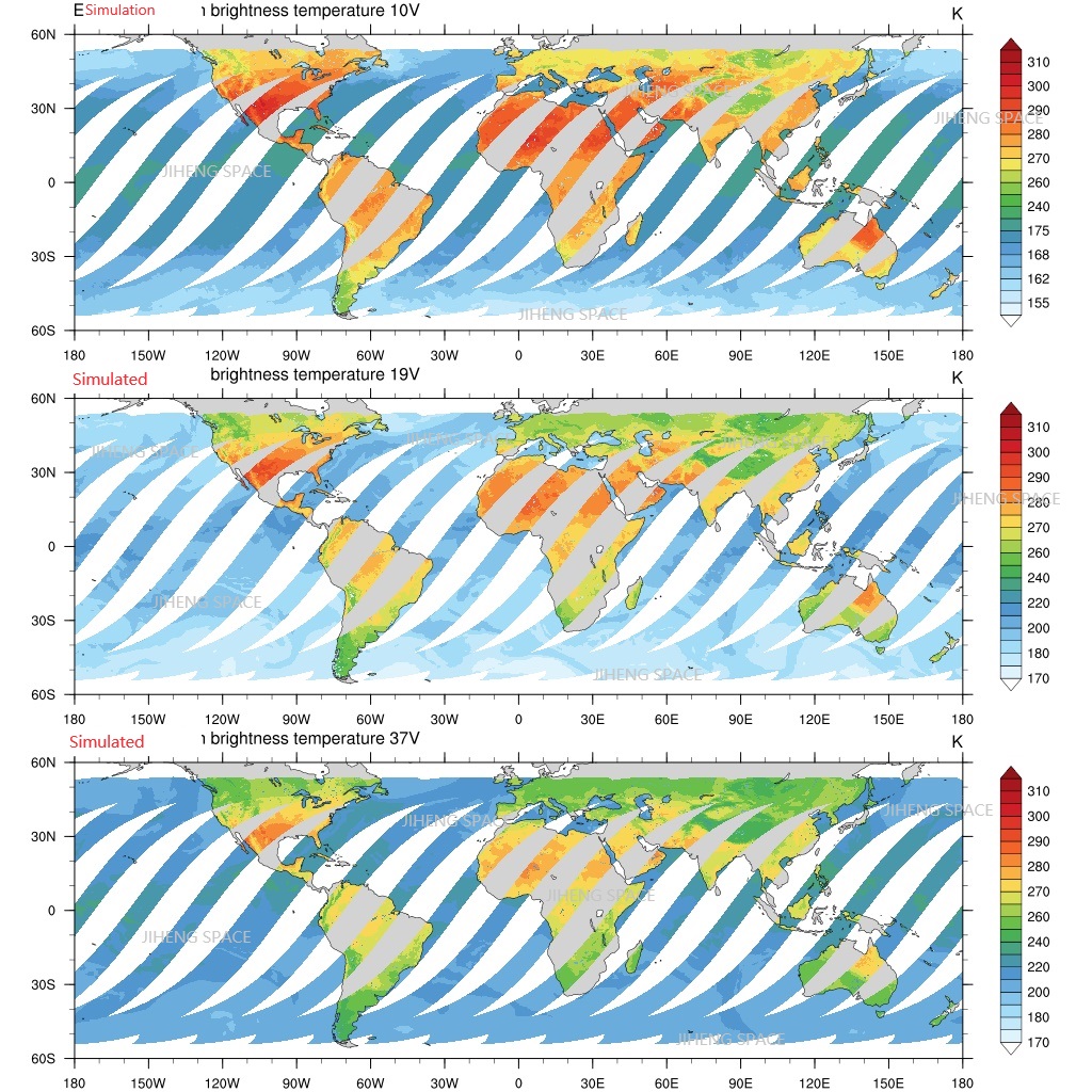
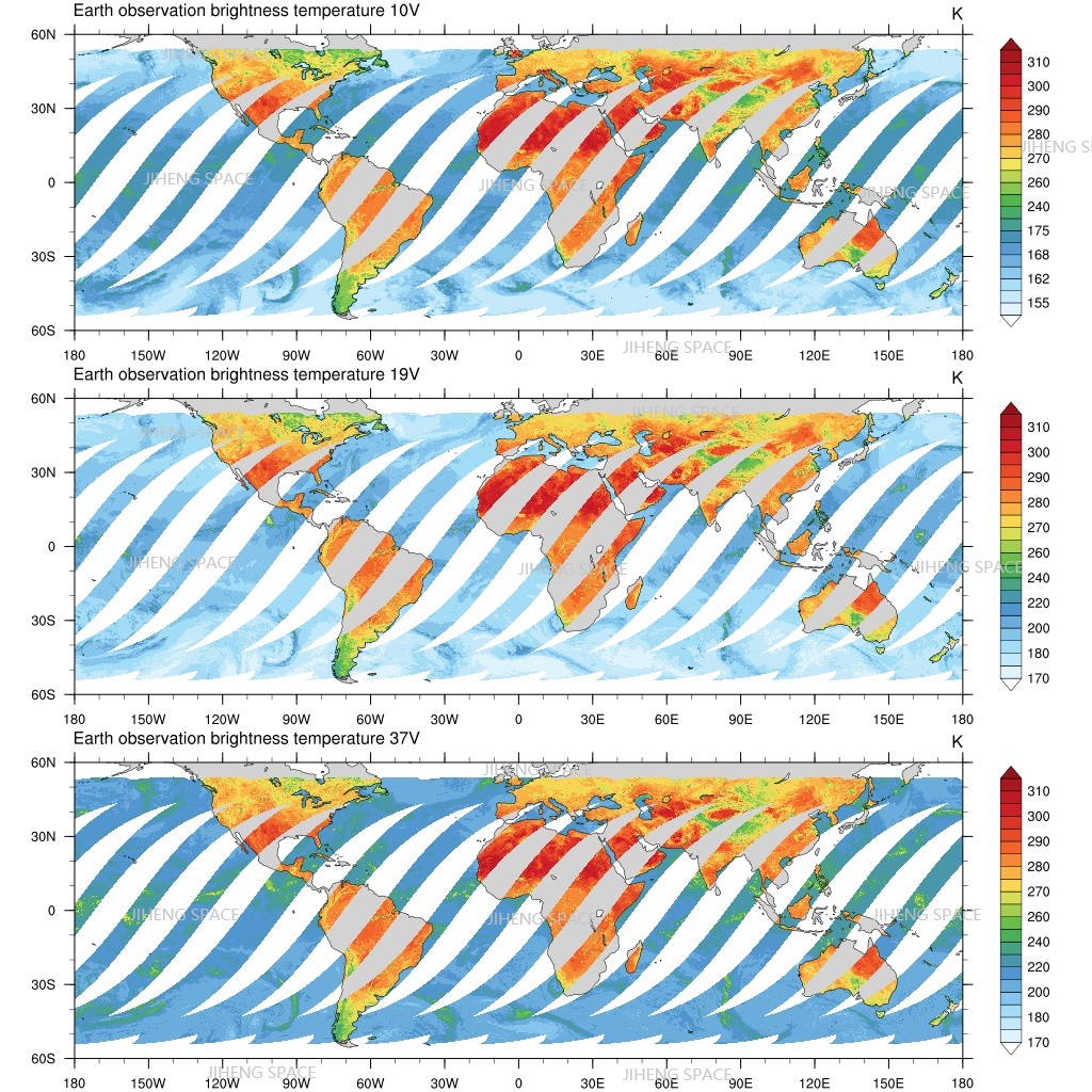
可以看出,两者在海陆、森林、沙漠、草地等区域的分布格局是一致的,比如亚马逊雨林中等,沙漠是高值,青藏高原是低值。
但是,两者在细节上存在较为明显的差异:陆面上模拟值显著偏低;洋面和漠北存在细节没有模拟出来。这可能的原因包括地表温度、地表发射率的模拟误差和以及没有考虑云的影响。在后面的章节我们会作这方面的模拟。


个例实战(三) 使用Emissvity Atlas

本个例个例二的设置和假设基本一致,只不过我们会使用TELSEM2的EmissivityAtlas来替换原有的模拟自己计算的emissivtity。

下载TELSEM2 Atlas

下载页:https://nwp-saf.eumetsat.int/site/software/rttov/download/#Emissivity_BRDF_atlas_data
下载telsem2_mw_atlas.tar.bz2解压在/home/hjh/rttov13/emis_data/目录下:

bash
$ cd /home/hjh/rttov13/emis_data
$ tar -xvf telsem2_mw_atlas.tar.bz2
├── ssmi_mean_emis_climato_01_cov_interpol_M2
├── ssmi_mean_emis_climato_02_cov_interpol_M2
├── ssmi_mean_emis_climato_03_cov_interpol_M2
├── ssmi_mean_emis_climato_04_cov_interpol_M2
├── ssmi_mean_emis_climato_05_cov_interpol_M2
├── ssmi_mean_emis_climato_06_cov_interpol_M2
├── ssmi_mean_emis_climato_07_cov_interpol_M2
├── ssmi_mean_emis_climato_08_cov_interpol_M2
├── ssmi_mean_emis_climato_09_cov_interpol_M2
├── ssmi_mean_emis_climato_10_cov_interpol_M2
├── ssmi_mean_emis_climato_11_cov_interpol_M2
├── ssmi_mean_emis_climato_12_cov_interpol_M2
├── telsem2
│   ├── Makefile
│   ├── mod_mwatlas_m2.F90
│   ├── README_TELSEM2.pdf
│   ├── readme.txt
│   └── test_telsem2.F90
└── correlations

telsem包含了ASCII方式存储的Atlas和独立的Fortran读取代码,可以在别的地方使用。RTTOV内置了针对TELSEM2的发射率地图和相应的插值工具的支持。

使用Atlas

fortran
根据提供的月份读取emissivity
! Use emissivity atlas
CALL rttov_get_emis( &
errorstatus, &
opts, &
chanprof, &
profiles, &
coefs, &
emis_atlas, &
emissivity(:) % emis_in)

如果是海洋或者没有telsem2 atlas的地方,使用RTTOV地表模式进行计算:

fortran
example_atlas_fwd.F90
! Calculate emissivity within RTTOV where the atlas emissivity value is zero or less
calcemis(:) = (emissivity(:) % emis_in <= 0._jprb)
! Use the RTTOV emissivity calculations over sea surfaces
DO j = 1, SIZE(chanprof)
IF (profiles(chanprof(j)%prof) % skin % surftype == surftype_sea) THEN
calcemis(j) = .TRUE.
ENDIF
ENDDO

调用RTTOV进行计算:

fortran
example_atlas_fwd.F90
CALL rttov_direct(                &
errorstatus, &! out error flag
chanprof, &! in channel and profile index structure
opts, &! in options structure
profiles, &! in profile array
coefs, &! in coefficients structure
transmission, &! inout computed transmittances
radiance, &! inout computed radiances
calcemis = calcemis, &! in flag for internal emissivity calcs
emissivity = emissivity, &! inout input/output emissivities per channel
calcrefl = calcrefl, &! in flag for internal BRDF calcs
reflectance = reflectance) ! inout input/output BRDFs per channel

RTTOV计算的地表发射率:
RTTOV计算的地表发射率

RTTOV计算的地表发射率

Fastem海表发射率模拟+TELSEM2地表发射率
RTTOV计算的地表发射率

RTTOV计算的地表发射率

晴空亮温模拟(TELSEM2 Atlas提供地表发射率)

参数的敏感性研究

略。有时间的话补充,计划交给师妹练手。

经验

  1. 在进行轨道模拟的时候,如果内存允许,应当将模拟样本一次性输入RTTOV中,这比循环每次样本并调用一次接口快很多。RTTOV的每次运行需要先inital,allocate, deallocate, check profile, check coefficents,等一系列的流程。频繁的结构体的创建、检查、赋值、释放,消耗绝大部分的时间;并且Fortran(formula transform)的优势就是进行快速的矩阵运算,所以大批量的数据一次性计算效率非常高。
    在本个例中,单个样本的循环模拟的方案下,完成一轨的模拟[294,1640]需要消耗约3小时;而逐Scan的模拟只需要3~4分钟,这其中约有2分钟用来下载数据。当然了,还可以整轨一次模拟(需要转成一维),这样会更快,但是需要恢复输出值的轨道形状,比较麻烦。如果后续速度成为卡脖子问题(目前已经很快了,不做循环迭代的情况下),再进行优化。