Geometry and the Discrete Fourier Transform
We'll show a relationship between some elementary geometry
of the plane and the Discrete Fourier Transform, that is a starting point for
ramifications for polynomials, circulant matrices and interpolation, and even sculpture.
We employ some recent technology to do this.
...
Patrick D. F. Ion
Mathematical Reviews
ion at ams.org
Geometry and the Discrete Fourier Transform
Patrick D. F. Ion
Mathematical Reviews
ion at ams.org
Introduction
Many of the most curious and popular theorems of plane geometry
are those of Coincidence, Collinearity, and Equilateralness (also
sometimes called Equilaterality):
a certain collection of lines all intersect in a
single point, or a collection of points in
the plane lies on a line, or a certain triple of points form an equilateral triangle.
The Discrete Fourier Transform is a tool
used to efficiently and accurately
approximate the Fourier Transform. It is applied
in electrical engineering to analyze
a signal into its components at various frequencies, and in mechanical
engineering to analyze vibrations of a system.
There is a surprising connection between
these two topics.
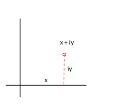
The starting point is to consider
points in the plane as complex numbers $z = x+\ii y\in\cplx.$
To see a note on new technology behind this document, and explanation of the buttons above, click on
the following up-arrow; to hide it again click on the corresponding down-arrow when it is shown
.
This pairing of up- and down-arrows is used to Show or Hide asides or details of equations.
Part I. The theorems
Theorems of Coincidence: Triangle Medians
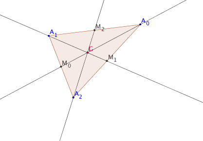
The median lines of a triangle are the lines drawn
from each vertex to the mid-point of the opposite side.
The simplest Coincidence Theorem asserts that these three lines meet in
a single point (which happens to be the center of gravity or centroid of the triangle).
There are other well known examples: the angle bisectors all intersect at the point
$I$, the center of the inscribed circle
(called the incenter), the perpendicular bisectors of the sides intersect at
the circumcenter $C$, the altitudes intersect at the orthocenter $O$.
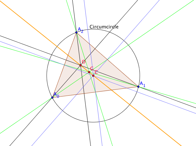
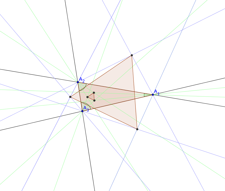
Collinearity theorems
The prime example of a collinearity theorem is that the circumcenter $C$, the centroid $G$
and the orthocenter $O$ are collinear.
Below the altitudes are in black, medians are in green and perpendicular bisectors in blue.
The line through their coincidence is shown in orange.
Equilateralness - Napoleon's Theorem
Napoleon's theorem, though probably not directly due to the emperor
himself, has long borne his name.
Its simplest form
says that if one constructs an equilateral triangle external to each side
of a nondegenerate plane triangle, and takes the three centroids of
the resulting triangles, then these points form an equilateral
triangle.
A similar construction
using internal triangles also leads to another equilateral triangle.

The most famous equilaterality theorem is Morley's Miracle from about 1901
which states that the pairwise intersections of adjacent internal angle trisectors
are the vertices of an equilateral triangle.
In the case shown there is the equilateral triangle from the internal trisectors, and
another one from external trisectors is show as well. The internal
trisectors are shown in green, the external trisectors are shown in
lilac.
A pentagon construction
A relatively recent construction was discovered by
the Fields Medalist Jesse Douglas. It was devised probably around 1940,
but only published in 1960, in a piece written in honor of a colleague Jekuthiel Ginsburg.
He specifies a fixed construction that from
any pentagon derives an associated convex pentagon and pentagram.
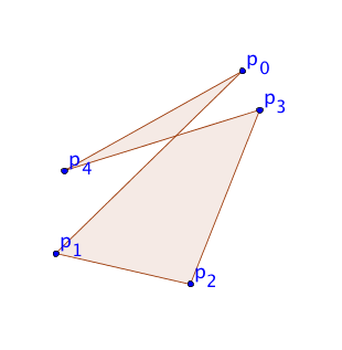
Consider a pentagon in the plane. Suppose the five vertex points are $ p_0, p_1, p_3
p_3, p_4$, taken to be numbers in $\cplx$.
So we are given a complex vector in $\cplx^5$, which is to say an array of complex numbers
$$ p=(p_0,p_1,p_2,p_3,p_4).$$
No one point of the five is to be distinguished.
What is important is the cyclic order,
so we shall consider the indices $i$
of $p_i$ modulo $5$. Sums in the index are cyclic, so that, for instance, $p_{3+4} = p_2$.
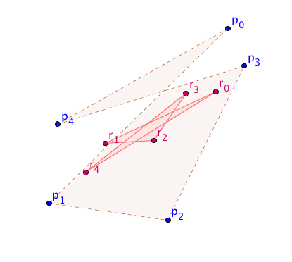
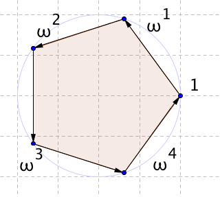
Douglas tells us: Join each vertex $p_i$ to the midpoint of the edge opposite between the
points $p_{i+2}$ and $p_{i+3}$; then extend that line by an extra
$(1/\sqrt{5})$ of its length to create a new vertex $q_i$.
The new pentagon $(q_0,q_1, q_2, q_3, q_4)$ is always the affine image of a convex regular
pentagon. Also, if the lines to the opposite midpoints are shortened
by a similar decrement of $(1/\sqrt{5})$ to give new vertices $r_i$, then
$(r_0, r_1, r_2, r_3, r_4)$ is the affine image of a regular star pentagon,
commonly called a pentagram.
We plot a chosen example of $p=(p_0,p_1,p_2,p_3,p_4)$ but,
as usual, the vertices can be dragged about in the interactive pop-up figures.
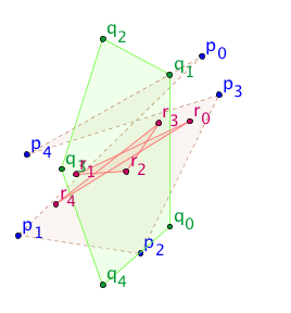
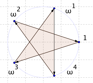
We see
$$
q_i = p_i + \left(1+{\textstyle\sfrac1{\sqrt{5}}}\right)
\left({{\textstyle\sfrac12}}(p_{i+2}+p_{i+3}) - p_i\right) ,
$$
outlined in green in the figure.
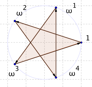
and similarly
$$
r_i = p_i + \left(1-{\textstyle\sfrac11{\sqrt{5}}}\right)\left({\textstyle\sfrac12}(p_{i+2}+p_{i+3}) - p_i\right) ,
$$
outlined in red.
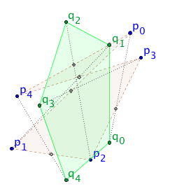
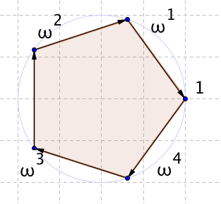
One may put all this in a diagram with evrything drawn, which it is amusing to pull about to see
the effect of the construction.
We see that starting from an arbitrary pentagon, a list of five points, we get by a fixed
construction two new pentagons, which are, respectively, an affine image of a standard
convex pentagon and an affine image of a standard pentagram.
Aside: affine transformations
Affine transformations
The general form of an affine transformation of the plane
with coordinates $x$ and $y$, can be written
$$\left(\begin{array}{c}x\\
y\\ \end{array}\right)
\mapsto
\left(\begin{array}{cc}a&b\\
c&d\\ \end{array}\right)
\left(\begin{array}{c}x\\
y\end{array}\right) +
\left(\begin{array}{c}e\\
f\end{array}\right)
.$$
If we view the $(x,y)$-plane as the complex plane $\cplx$, thus in
terms of $z=x+\ii y$ with $\ii = \sqrt{-1}$, we have to translate
the above into complex language.
We see the general plane affine transformation written in complex
coordinates is
$$
z \mapsto \lambda z + \mu \overline z + \nu
$$
with $2 \lambda=(a+d)+(c-b)\ii,\ 2 \mu=(a-d)+(c+b)\ii,\ \nu\in\cplx$.
The addition of a constant term can
be realized by the addition of a complex number:
$$z = x + \ii y \mapsto x + \ii y + (e + \ii f)$$ so we are left with the
matrix to deal with.
Since in the above affine transformation $x$ and $y$ are not
coupled, a moment's reflection reveals that the expression using
complex coordinates for an affine transformation will have to
involve both $z$ and $\overline z$, the complex conjugate, so as to
provide access to the real and imaginary parts of $z$. But then we
just need to equate the general forms
$$(\alpha + \ii \beta) (x + \ii y) + (\gamma + \ii \delta) (x - \ii y)
= (ax + by) + \ii (cx + dy) .$$
The solution is
$$\left(\begin{array}\alpha\\
\beta\\ \gamma\\ \delta\\\end{array}\right)
= {1\over2}
\left(\begin{array}{c}a+d\\ c-b\\ a-d\\ c+b\\\end{array}\right)
={1\over2}
\left(\begin{array}{cccc}1&0&0&1\\ 0&-1&1&0\\
1&0&0&-1\\ 0&1&1&0\end{array}\right)
\left(\begin{array}{c}a\\ b\\ c\\ d\\\end{array}\right).
$$
So we see the general plane affine transformation written in complex
coordinates is
$$
z \mapsto \lambda z + \mu \overline z + \nu
$$
with $2 \lambda=(a+d)+(c-b)\ii,\ 2 \mu=(a-d)+(c+b)\ii,\ \nu\in\cplx$.
Another way of seeing this is just to note that the change from real to
complex coordinates is
\begin{eqnarray*}
\left(\begin{array}{c} x\\
y\\ \end{array}\right)
&=&
\left(\begin{array}{c} (z+\zbar)/2\\
(z-\zbar)/2\ii\\ \end{array}\right)
=\frac12
\left(\begin{array}{cc} \ \ 1&\ 1\\
-\ii&\ii\\ \end{array}\right)
\left(\begin{array}{c} z\\
\zbar\\ \end{array}\right) \\
&\mapsto&\frac12
\left(\begin{array}{cc} a&b\\
c&d\\ \end{array}\right)
\left(\begin{array}{cc} \ 1&\ 1\\
-\ii&\ii\\ \end{array}\right)
\left(\begin{array}{c} z\\
\zbar\\ \end{array}\right)
=\frac12
\left(\begin{array}{cc} a-\ii b& a+\ii b\\
c-\ii d& c+\ii d\\ \end{array}\right)
\left(\begin{array}{c} z\\
\zbar\\ \end{array}\right). \\
\end{eqnarray*}
In other words
\begin{eqnarray*}
\left(\begin{array}{c} z\\
\zbar\\ \end{array}\right)
= &\mapsto&\frac12
\left(\begin{array}{cc} \ 1& +\ii\\
\ 1&-\ii\\ \end{array}\right)
\left(\begin{array}{cc} a&b\\
c&d\\ \end{array}\right)
\left(\begin{array}{cc} \ 1&\ 1\\
-\ii& +\ii\\ \end{array}\right)
\left(\begin{array}{c} z\\
\zbar\\ \end{array}\right) \\
& =& \frac12
\left(\begin{array}{cc} \ 1& +\ii \\
\ 1& -\ii \\ \end{array}\right)
\left(\begin{array}{cc} a-\ii b& a+\ii b\\
c-\ii d&c+\ii d\\ \end{array}\right)
\left(\begin{array}{c} z\\
\zbar\\ \end{array}\right) \\
& =& \frac12
\left(\begin{array}{cc} (a+d)-(b-c)\ii & (a-d)+(b+c)\ii\\
(a-d)-(b+c)\ii & (a+d)+(b-c)\ii\\ \end{array}\right)
\left(\begin{array}{c} z\\
\zbar\\ \end{array}\right),\\
& =&
\left(\begin{array}{cc} \lambda & \mu\\
\overline{\lambda} & \overline{\mu}\\ \end{array}\right)
\left(\begin{array}{c} z\\ \zbar\\ \end{array}\right),\\
\end{eqnarray*}
since
$$ \frac12
\left(\begin{array}{cc} \ 1&+\ii \\
\ 1&-\ii \\ \end{array}\right)
\left(\begin{array}{cc} \ 1&\ 1\\
-\ii&+\ii\\ \end{array}\right)
=
\left(\begin{array}{c} \ 1&\ 0\\
\ 0&\ 1\\ \end{array}\right).
$$
Now consider the case of a linear sum of a regular $n$-gon and
its opposite, say the case of the convex pentagon where we had $n=5$.
The points are of the form $A \omega^k + B \omega^{-k}$. But
$\omega^{-1}=\bar \omega$, so these points are affine images of the
points of the standard convex pentagon with parameters
$$
(\lambda,\mu,\nu) = (A, B, 0).
$$
That's what we have above as the result of Douglas's construction with a similar
consideration for the affine image of a standard pentagram.
Part II. Geometry with the Discrete Fourier Transform
The Discrete Fourier Transform
A polygon with $N$ sides is a sequence of vertices $p_{0}$, $p_{1}$, ... , $p_{N-1}$.
None of the vertices is particularly more important than the others, so all that
really matters is the cyclic order. In other words, what we have at hand
is a complex-valued function $p_{j}$ on the cyclic group $\intg/N$
(short for $\intg/N\intg$.
The vector space $\cplx[\intg/N]$ of all complex-valued functions on $\intg/N$ has dimension $N$,
and the natural coordinate system on this space assigns to a function $f$ the array
$(f_{0}, \dots , f_{N-1})$ in $\cplx^{N}$. But there is another
useful coordinate system as well. To tell you what this is,
we need to specify a new basis of the vector space.
Let $\omega_{N} = \ee^{2 \pi \ii/N}$, and
for each $a$ in $\intg$, let $\chi_{a}$ (more precisely $\chi_{N,a}$) be the function taking
$j$ to $\omega_{N}^{aj}$. This is a function on
$\intg/N$, since $\omega_{N}^{N} = 1$, that is $\omega_{N}$ is an $N$-th root of unity.
Furthermore, $\chi_{a}$ only depends on $a$ modulo $N$, so there are
$N$ of these functions.
We assign to the complex vector space of complex-valued functions on $\intg/N$ a
a Hermitian inner product:
$$ p \Dot q = { 1 \over N} \sum_{j=0}^{N-1} p_{j}\bar{q}_{j}
= (1/N)(p_{0}\bar{q}_{0} + \cdots + p_{N-1}\bar{q}_{N-1}) . $$
The function $\chi_{0}$ is just the constant function taking all $j$ to $1$.
We have
$$ \chi_{a} \Dot \chi_{0} = \begin{cases}
1 \text{ if } a=0 \cr
0 \text{ otherwise} \cr
\end{cases} $$
and hence
$$ \chi_{a} \Dot \chi_{b} = \begin{cases}
1 \text{ if } a=b \cr
0 \text{ otherwise.}\cr
\end{cases} $$
This means that the functions $\chi_{a}$ for $a$ in $\intg/N$
are an orthonormal basis for the space of functions on
$\intg/N$. If $f$ is any such function, we may therefore write
$$ f = \sum_{a=0}^{N-1} \hat{f}_{a} \chi_{a} \quad \text{ where } \quad \hat{f}_{a} = f \Dot \chi_{a} $$
In particular, $\hat f_{0}$ is the center of gravity
(a.k.a. centroid, barycenter or mean) of the values of $f$,
$$
\hat{f}_{0} = \frac{1}{N} (f_0 + \cdots + f_{N-1})
$$
and
$\hat{f}_{0},\dots,\hat{f}_{N-1}$ are the coefficients in the
expression of the arbitrary function $f$, an $N$-gon, as a linear sum of standard
ones.
For example, the function $f_{j} = \chi_{1}(j)$ lists the vertices
of the symmetric regular polygon of $N$ sides inscribed in
the unit circle.
Similarly $g_{j} = \chi_{N-1}(j)$ gives the standard negatively
oriented unit $N$-gon. The combination
$\lambda \chi_{1} +\mu \chi_{N-1}$ with $\lambda$, $\mu$ in $\cplx$ then gives a general
affine convex $N$-gon.
Triangle geometry
The claim is that much classical plane geometry has a
natural expression from the point of view outlined above. Start
by looking at the standard types of triangles. For that we'll take
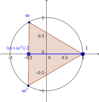
$\omega := \omega_3^{\strut} = \frac12(-1 + \ii \sqrt3)$ until further notice.
The standard triangles are $\chi_0=(1,1,1)$, the degenerate one with 3 points at 1,
the unit equilateral triangle $\chi_1=(1,\omega,\omega^2)$,
and its reverse $\chi_2=(1,\omega^2,\omega)$.
The picture below shows the simple average of a standard equilateral
triangle and its reverse, namely $\sfrac12(\chi_1+\chi_2)$.
It is a digon (a segment) with a double point at the left-hand end.
We consider only triangles
whose centroids are at the origin; after all, it is easy enough to move any triangle
into this simplifying position by a translation, and all interesting theorems of
plane geometry are invariant under translations.
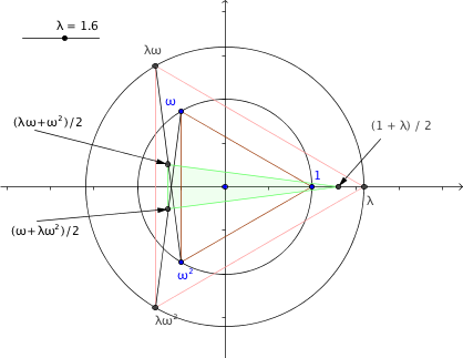
If we
separate the two triangles by making the standard one larger, say lying on a circle of
radius $\lambda>1$ then we get
which shows the triangle is an isosceles one with height $\sfrac34(\lambda+1)$
lying along the real axis.
The slider labelled $\lambda$ controls the radius of the outer circle.
The green isosceles triangle in the middle is the
average of the two triangles with labelled vertices. Note the opposite
orientations of the two triangles being averaged.
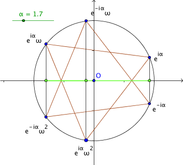
If we separate the two basic triangles $\chi_1$ and $\chi_2$ by
turning them in opposite directions by a turn $\ee^{\ii \alpha}$ (in
the attractive terminology of Frank Morley for complex numbers of modulus 1) to make
$$
\begin{eqnarray}
{\textstyle\sfrac12}(\ee^{\ii \alpha}\chi_1+\ee^{-\ii \alpha}\chi_2)&=&
{\textstyle\sfrac12}\left\{\ee^{\ii \alpha}(1,-{\textstyle\sfrac12}+{\textstyle\sfrac{\sqrt3}2}\ii,
-{\textstyle\sfrac12}-{\textstyle\sfrac{\sqrt3}2}\ii)
+\ee^{-\ii \alpha}(1,-{\textstyle\sfrac12}-{\textstyle\sfrac{\sqrt3}2}\ii,
-{\textstyle\sfrac12}+{\textstyle\sfrac{\sqrt3}2}\ii)\right\}\cr
&=& \left({\textstyle\sfrac12}(\ee^{\ii \alpha}+\ee^{-\ii \alpha}),
-{\textstyle\sfrac14}(\ee^{\ii \alpha}+\ee^{-\ii \alpha})+
{\textstyle\sfrac{\sqrt3}4}\ii(\ee^{\ii \alpha}-\ee^{-\ii \alpha})
,-{\textstyle\sfrac14}(\ee^{\ii \alpha}+\ee^{-\ii \alpha})-
{\textstyle\sfrac{\sqrt3}4}\ii(\ee^{\ii \alpha}-\ee^{-\ii \alpha})\right)\cr
&=&(\cos \alpha,
-{\textstyle\sfrac12}\cos \alpha-{\textstyle\sfrac{\sqrt3}2}\sin \alpha,
-{\textstyle\sfrac12}\cos \alpha+{\textstyle\sfrac{\sqrt3}2}\sin \alpha)
)
\end{eqnarray}
$$
$$
\begin{eqnarray}
{\textstyle\sfrac12}(\ee^{\ii \alpha}\chi_1+\ee^{-\ii \alpha}\chi_2)=
(\cos \alpha,
-{\textstyle\sfrac12}\cos \alpha-{\textstyle\sfrac{\sqrt3}2}\sin \alpha,
-{\textstyle\sfrac12}\cos \alpha+{\textstyle\sfrac{\sqrt3}2}\sin \alpha)
)
\end{eqnarray}
$$
then we have achieved a splitting of the double point at $-\sfrac12$
in $\sfrac12(\chi_1+\chi_2)$ but still have a degenerate triangle on
the real axis, with the second vertex at $z_1=-\sfrac12\cos
\alpha-\sfrac{\sqrt3}2\sin \alpha$ and the third symmetrically
placed about $-\frac12\cos\alpha$ at $z_2=-\sfrac12\cos
\alpha+\sfrac{\sqrt3}2\sin \alpha$.
The green slider $\alpha$ controls the angle away from the $x$-axis that the triangles are rotated;
it goes from $0$ to $2 \pi$.
The linear green triangle is the average of the triangles with
vertices on the unit circle. Note that the cycle $\ee^{\ii\alpha}$, $\ee^{\ii\alpha}\omega$
and $\ee^{\ii\alpha}\omega^2$ is positively oriented (counter-clockwise)
and $\ee^{\ii\alpha}$, $\ee^{\ii\alpha}\omega^2$
and $\ee^{-\ii\alpha}\omega$ is negatively oriented.
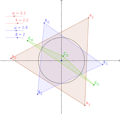
The fully general case is then the addition of two arbitrarily sized and rotated
standard triangles. This is a case where the interactive form of the diagram can
be quite helpful.
The triangle $C$ is the average of triangles $A$ and $B$ so $C_i$ is midway
between $A_i$ abd $B_i$. That is $C$ is the triangle
${\scriptstyle\frac12}(\lambda \ee^{\ii \alpha}\chi_1 +\mu \ee^{\ii \beta}\chi_2)$.
The red sliders are $\lambda$ controlling the size of the red image of the standard triangle and
$\alpha$ controlling its angle of rotation. Then the blue $\mu$ and $\beta$ are the corresponding controls
for the blue image of the reversed standard triangle.
The general sum of this form, with six real parameters
$\lambda,\mu,\nu,\alpha,\beta,\gamma\in \reals$, is
$$
\lambda \ee^{\ii \alpha}\chi_1 +\mu \ee^{\ii \beta}\chi_2 +
\nu \ee^{\ii \gamma}\chi_0
$$
and can represent any triangle in the plane; the centre of gravity is
$\nu \ee^{\ii \gamma}\chi_0$.
One can spend quite some time playing with the interactive figures for polygon
superpositions.
Proof of Median Coincidence
If the vertices of a triangle are $z=(z_0,z_1,z_2)$, the midpoints
of the sides are
$$$$
where $I$ is the identity and $J$ is the cyclic permutation
$$
J: (z_0,z_1,z_2) \mapsto (z_1,z_2,z_0) .
$$
The points on the line from $z_0$ to $\sfrac12(z_2+z_1)$ are of the form,
for some $\lambda \in \reals$
$$
(1-\lambda)z_0 + \lambda {\textstyle\sfrac12}(z_2+z_1)
$$
and similarly on the line from $z_1$ to $\sfrac12(z_0+z_2)$ we have,
for some $\mu \in \reals$
$$
(1-\mu)z_1 + \mu {\textstyle\sfrac12}(z_0+z_2).
$$
The only solution for a point that lies on both lines is
$$
(1-{\textstyle\sfrac23})z_1 + {\textstyle\sfrac23}{\textstyle\sfrac12}(z_0+z_2) =
{\textstyle\sfrac13}(z_0 + z_1 + z_2) = \chi_0 \Dot z.
$$
The common intersection point of medians as the centre of gravity has become obvious.▓
Proof of other coincidences and collinearity
Other coincidence cases can be a bit more tricky but fundamentally proceed
in a similar way. We need to show the Fourier transform coefficients of $\chi_1$ and
$\chi_2$ both vanish. For collinearity we only need to show that
$ \chi_1 \Dot x$ and $ \chi_2 \Dot x $ have the same absolute value.
Pentagon geometry and Jesse Douglas' pentagon construction explained
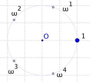
Let $\omega$ be the simplest primitive $5$th root of unity, with $\ii := \sqrt{-1}$:
$$
\omega = \cos\frac {2\pi}{5} + \ii \sin\frac {2\pi}{5}.
$$
Note that complex conjugation
acts as $\bar{\omega}_5^j = \omega_5^{5-j}$.
These are the 5 standard vectors
$$
\chi_0=(
1,
1,
1,
1,
1
)
\quad;\quad
\chi_1=(
1,
\omega_5^\strut,
\omega_5^2,
\omega_5^3,
\omega_5^4
)
\quad;\quad
\chi_2=(
1,
\omega_5^2,
\omega_5^4,
\omega_5^\strut,
\omega_5^3
)
\quad;\quad
\chi_3=(
1,
\omega_5^3,
\omega_5^\strut,
\omega_5^4,
\omega_5^2
)
\quad;\quad
\chi_4=(
1,
\omega_5^4,
\omega_5^3,
\omega_5^2,
\omega_5^\strut
).
$$
which form a basis for $\cplx^5$.
Remark also that
$$\cos\frac{2}{\pi}5 = \cos 72^\circ = \frac{1}{4} (-1+\sqrt5)\simeq 0.309, \quad \sin\frac{2}{\pi} 5
=\cos 18^\circ = \frac{1}{4}\sqrt{10+2\sqrt5} \simeq 0.951 .
$$
In fact, in terms of square roots,
$$
\left(
\begin{array}{c}
1\\
\omega_5^{\phantom{1}}\\
\omega_5^2\\
\omega_5^3\\
\omega_5^4
\end{array}\right) =
\frac{1}{4}
\left(
\begin{array}{c}
4\\
-1+\sqrt5 + \ii \sqrt{10+2\sqrt5}\\
-1-\sqrt5 + \ii \sqrt{10-2\sqrt5}\\
-1-\sqrt5 - \ii \sqrt{10-2\sqrt5}\\
-1+\sqrt5 - \ii \sqrt{10+2\sqrt5}
\end{array}
\right)
$$
$$=
\frac{1}{4} \left\{\, \left[
-\left(
\begin{array}{c}
1\\
1\\
1\\
1\\
1
\end{array}
\right)
+\sqrt5\,
\left(
\begin{array}{c}
\sqrt5\\
+1\\
-1\\
-1\\
+1
\end{array}
\right)
\,\right] +
\frac{\ii}{2} \sqrt{10+2\sqrt5}\,
\left[\,\,
\left(
\begin{array}{c}
0\\
2\\
1\\
-1\\
-2
\end{array}
\right)
+\sqrt5\,
\left(
\begin{array}{c}
0\\
0\\
-1\\
1\\
0
\end{array}
\right) \,
\right]\, \right\}
$$
which seems complicated enough.
Going back to examine the coordinates for $q_i$, the point got by extending
a line from a vertex to an opposite mid-point by an extra $\frac1{\sqrt5}$, we see
$$q_i = -\frac{\sqrt5}5 p_i + \frac{5+\sqrt5}{10} p_{i+2}+ \frac{5+\sqrt5}{10} p_{i+3}.$$
To establish properties see what components of the various standard types it has.
The function $q=(q_0,q_1,q_2,q_3,q_4))\in{\cplx}[{\intg}/5]$ has the harmonic expansion
q = \sum_{k=0}^{4} (\chi_k \Dot q) \chi_k = \sum_{k=0}^{4}\hat q_k \chi_k.
$$
The character $\chi_0$ is the trivial (or degenerate) character of the
trivial representation, and
$\hat f_{0}$ is the center of gravity of the values of $f$. The other
$\hat f_{1},\hat f_{2},\hat f_{3},\hat f_{4}$ are the harmonic components
of $f$.
The center of gravity is just an expression of where the geometric object is located,
so we don't expect any special properties for it. But look at $\hat q_2$; we find
by calcualtion
$$
\begin{eqnarray}
5\hat {q_2}=5 \chi_2 \Dot q = 0\end{eqnarray}
$$
$$
\begin{eqnarray}
5\hat {q_2} &=&5 \langle \chi_2 | q\rangle \\
&=& 1\cdot q_1 + \overline{ \omega_5^{2}}\cdot q_2 + \overline{ \omega_5^{4}}\cdot q_3 +
\overline{ \omega_5^{1}}\cdot q_4 + \overline{ \omega_5^{3}}\cdot q_5\\
&=& q_1 +\omega_5^{3} q_2 + \omega_5^{1} q_3 + \omega_5^{4} q_4 + \omega_5^{2} q_5\\
&=& -\frac{\sqrt5}5( p_1 +\omega_5^{3} p_2 + \omega_5^{1} p_3 + \omega_5^{4} p_4 +
\omega_5^{2} p_5) +\\
& & \frac{5+\sqrt5}{10}( p_3 +\omega_5^{3} p_4 + \omega_5^{1} p_5 + \omega_5^{4} p_1 +
\omega_5^{2} p_2) +\\
& & \frac{5+\sqrt5}{10}( p_4 +\omega_5^{3} p_5 + \omega_5^{1} p_1 + \omega_5^{4} p_2 +
\omega_5^{2} p_3)\\
&=& (-\frac{\sqrt5}5\cdot1 + \frac{5+\sqrt5}{10} \omega_5^{4} +
\frac{5+\sqrt5}{10} \omega_5^{1})p_1 +\\
& & (-\frac{\sqrt5}5 \omega_5^{3} + \frac{5+\sqrt5}{10} \omega_5^{2} +
\frac{5+\sqrt5}{10} \omega_5^{4})p_2 +\\
& & (-\frac{\sqrt5}5 \omega_5^{1} + \frac{5+\sqrt5}{10} \cdot1 +
\frac{5+\sqrt5}{10} \omega_5^{2})p_3 +\\
& & (-\frac{\sqrt5}5 \omega_5^{4} + \frac{5+\sqrt5}{10} \omega_5^{3} +
\frac{5+\sqrt5}{10} \cdot1)p_4 +\\
& & (-\frac{\sqrt5}5 \omega_5^{2} + \frac{5+\sqrt5}{10} \omega_5^{1} +
\frac{5+\sqrt5}{10} \omega_5^{3})p_5 .
\end{eqnarray}
$$
The thing to note is that the coefficients of the points $p_i$ are all
multiples by powers of $\omega_5$ of the coefficient of $p_1$. Furthermore the
coefficient of $p_1$ is a real number since $\overline{\omega_5^{4}} = \omega_5^{1}$. But
$$
\begin{eqnarray}
- \frac{\sqrt5}5\cdot1 + \frac{5+\sqrt5}{10} \omega_5^{4} +
\frac{1+\sqrt5}{2}\omega_5^{1} =
-\frac{\sqrt5}5 + \frac{5+\sqrt5}{10}\left(\omega_5^{4} + \omega_5^{1}\right)
= 0 .
\end{eqnarray}
$$
$$
\begin{eqnarray}
- \frac{\sqrt5}5\cdot1 + \frac{5+\sqrt5}{10} \omega_5^{4} +
\frac{1+\sqrt5}{2}\omega_5^{1} &=&
-\frac{\sqrt5}5 + \frac{5+\sqrt5}{10}\left(\omega_5^{4} + \omega_5^{1}\right) \\
&=&
-\frac{\sqrt5}5 + \frac{5+\sqrt5}{10} 2 \Re{ \omega_5^{1}}
\\
&=&
-\frac{\sqrt5}5 + \frac{(5+\sqrt5)(-1+\sqrt5)}{10\times 2} \\
&=&
-\frac{\sqrt5}5 + \frac{-5+5-\sqrt5+5\sqrt5}{10\times 2} \\
&=&
-\frac{\sqrt5}5 + \frac{4\sqrt5}{20} = 0 .
\end{eqnarray}
$$
So $\hat q_2$ vanishes identically. Thus there is no regular pentagram
component of the polygon $q$. Similarly look at $\hat q_3$, or at
$$
\begin{eqnarray}
5\hat { q_3} = 5\ \chi_3 \Dot q = 5\ \overline{ \overline q\Dot\chi_2} = 0 .
\end{eqnarray}
$$
$$
\begin{eqnarray}
5\hat { q_3} &=& 5\ \langle \chi_3 | q\rangle \\
&=& 1\cdot q_1 + \overline{ \omega_5^{3}}\cdot q_2 + \overline{ \omega_5^{1}}\cdot q_3 +
\overline{ \omega_5^{4}}\cdot q_4 + \overline{ \omega_5^{2}}\cdot q_5\\
&=& q_1 +\omega_5^{2} q_2 + \omega_5^{4} q_3 + \omega_5^{1} q_4 + \omega_5^{3} q_5\\
&=& 5\ \overline{\chi_2} \Dot q \\
&=& 5\ \overline{ \overline q\Dot\chi_2} \\
&=& 0 .
\end{eqnarray}
$$
This is because the reason that $\chi_3 \Dot q = 0$ has little to do with
the properties of the $q_i$ as complex numbers, but was entirely the result of the
interaction between the $5$th roots of unity, and the real coefficients in the specific
make-up of the $q_i$ starting from arbitrary complex numbers $p_i$. If this
is unconvincing, then a similar argument to the previous one goes through but
involves the verification
$$
- \frac{\sqrt5}5\cdot1 + \frac{5+\sqrt5}{10} \omega_5^{1} + \frac{5+\sqrt5}{10}\omega_5^{4} = 0.
$$
We have thus shown that $q = {\hat q}_0 + {\hat q}_1 \chi_1 + {\hat q}_4\chi_4={\hat q}_0 +
{\hat q}_1 \chi_1 + {\hat q}_4 \overline{\chi_1}$. This means that $q$ is an affine image
of the regular convex pentagon.
Similarly the polygon $r$ constructed is the affine image of a regular pentagram,
for like reasons.
The pentagon $r$ has points given by
$$
r_i = \frac{\sqrt5}5 p_i + \frac{5-\sqrt5}{10} p_{i+2}+
\frac{5-\sqrt5}{10} p_{i+3}.
$$
For this case we examine correspondingly the
components ${\hat r}_1$ and ${\hat r}_4$. Again we can group the coefficients of
the points $p_i$, and see that they are all multiples of any one of them. For instance,
the coefficient of $p_1$ is
$$
\frac{\sqrt5}5\cdot1 + \frac{5-\sqrt5}{10} \omega_5^{2} + \frac{5-\sqrt5}{10} \omega_5^{3}=
\frac{\sqrt5}5 + \frac{5-\sqrt5}{10}\frac{-1-\sqrt5}{2} = 0,
$$
just as before, up to a couple
of sign changes. Also as before, we can conclude that ${\hat r}_1 = {\hat r}_4 = 0$, and say
that the polygon $r$ is the affine image of a regular pentagram. ▓
Proof of Napoleon's Theorem
Again take
$\omega := \omega_3^{\strut} = \frac12(-1 + \ii \sqrt3)$ until further notice,
so $\omega^3 - 1 = 0 = 1 + \omega + \omega^2.$
Start by expressing the construction steps in the
Napoleon theorem with the help of the characters we
introduced. We need to specify an equilateral triangle
constructed positively on an oriented segment. The standard unit
equilateral triangle is $\chi_{3,1}=:\chi_1$. Its right-hand vertex
is at the point $1\in\cplx$; we see that $\chi_1-\chi_0$ is a
similar triangle shifted so that its right-hand vertex is at the
origin. A diagram may help.
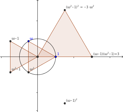
To shift it so that its first side is aligned positively along the
horizontal $x$-axis we multiply the whole by
$(\omega-1)^{-1}=3^{-1}(\omega^2-1)$ to get
$3^{-1}(\omega^2-1)(\chi_1-\chi_0)$.
This is clear because we want
to move the vertex after the base at $0$, namely at $\omega-1$, to
the point $1$, and
$$
(\omega -1)(\omega^2-1)=\omega^3-\omega^2-\omega+1=3.
$$
Alternatively, we see immediately that
$\overline{\omega-1}=\omega^2-1$ and $|\omega-1|=3$. The
triangular building block we need is thus
$$
3^{-1}(\omega^2-1)(\chi_1-\chi_0).
$$
There is an important thing to note about the constructed triangle:
it is positively oriented with respect to the base interval from $0$
to $1$. It is on the left as we go from $0$ to $1$. To get the
negatively oriented block on the right as we go from $0$ to $1$ we
need
$$
3^{-1}(\omega-1)(\chi_2-\chi_0).
$$
In general, to translate a whole triangular figure by a vector $z$
we have to add $z\chi_0$ to it.
To rotate by a angle $\alpha$ we
have to multiply by the scalar turn $\ee^{\ii\alpha}$, and to scale
by a homothety $\lambda > 0$ we have to multiply by the scalar
$\lambda$. For instance, if we had not multiplied by
$(\omega-1)^{-1}$ just a moment ago, but only used the rotation
effected by the unit vector
$\{3^{-1/2}(\omega-1)\}^{-1}=3^{-1/2}(\omega^2-1)$ then we would
have had to scale the building-block triangle to unit side-length by
multiplying with $3^{-1/2}$.
If the segment on which we need to erect a triangle is from $z_j$ to
$z_k$, then it is of length $|z_k-z_j|$ and in the direction
$\arg(z_k-z_j)$ from the starting point $z_j$. Thus the triangle
on the left side of the interval which is to be constructed is
$$
3^{-1}(\omega^2-1)(z_k-z_j)(\chi_1-\chi_0) + z_j\chi_0,
$$
and the triangle on the right side is
$$
3^{-1}(\omega-1)(z_k-z_j)(\chi_2-\chi_0) + z_j\chi_0.
$$
Finally, to find the centroid of a triangle
$z=(z_0,z_1,z_2)$ we just have to take the inner product with
$\chi_0$, namely $\chi_0 \Dot z$. So the centroid of the
left-side resulting triangle in the last paragraph is, using the
fact that the basis vectors $\chi_j$ are orthonormal,
\begin{eqnarray*}
\chi_0 \Dot( 3^{-1}(\omega^2-1)(z_k-z_j)(\chi_1-\chi_0) + z_j\chi_0)
&=& -3^{-1}(\omega^2-1)(z_k-z_j) + z_j\\
&=& -3^{-1}\{(\omega^2-1)z_k-(\omega^2-1)z_j-3z_j\}\\
&=& -3^{-1}\{(\omega^2-1)z_k-(\omega^2+2)z_j\}
.
\end{eqnarray*}
Theorem 1 (Napoleon)
For any nondegenerate triangle in the plane the result of
constructing the centroids of equilateral triangles erected
externally on the sides of the triangle is three points at the
vertices of an equilateral triangle.
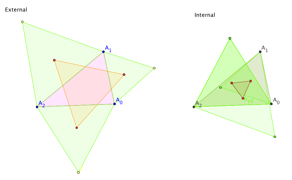
Proof. Let the initial triangle be $z=(z_0,z_1,z_2)$, and suppose
it positively oriented. Start with externally
constructed equilateral triangles. That means we need right-side
building blocks.
By the above remarks the externally constructed vertices are
$$
( -3^{-1}\{(\omega-1)z_{j+1}-(\omega+2)z_j\} , j\in \{0,1,2\}),
$$
so the triangle is
$$3
^{-1}\{(1-\omega)J z+ (\omega+2)z\}.
$$
To show that this is an equilateral triangle we take the
inner product with $\chi_2$. We know that the original triangle has
its Fourier decomposition $z=\hat z_0\chi_0+\hat z_1\chi_1+\hat
z_2\chi_2$, and the basis
$(\chi_j,j\in\{0,1,2\})$ is orthonormal. Now we see quickly that
the $\chi_j$ are eigenvectors of $J$, namely $J\chi_j = \omega^j\chi_J$.
Therefore $Jz=\hat z_0\chi_0+\omega \hat
z_1\chi_1+\omega^2 \hat z_2\chi_2$.
Thus
\begin{eqnarray*}
\langle\chi_2\Dot3^{-1}\{(1-\omega)J z+ (\omega+2)z\}\rangle
&=&3^{-1}\{(1-\omega)\omega^2 \hat z_2+ (\omega+2)\hat z_2\}\\
&=&3^{-1}\{\omega^2-1+\omega +2\}\hat z_2 \\
&=&3^{-1}\{\omega^2+\omega +1\}\hat z_2 \\
&=& 0.
\end{eqnarray*}
We have shown that constructing the centroids of
equilateral triangles externally to the positively oriented initial
triangle yields a sequence of points making up the vertices of a
positively oriented equilateral triangle.
To deal with left-hand side, i.e. , ‘internal’ equilateral
triangles, we just have to do a similar
calculation.
Since we may suspect that the resulting vertices will
have the reverse orientation we will take the inner product with
$\chi_1$.
As suspected, they are the vertices of a reverse equilateral triangle. ▓
Since we may suspect that the resulting vertices will
have the reverse orientation we will take the inner product with
$\chi_1$.
By remarks above the internally constructed vertices are
$$
( -3^{-1}\{(\omega^2-1)z_{j+1}-(\omega^2+2)z_j\} , j\in 0..2),
$$
so the triangle is
$$
3^{-1}\{(1-\omega^2)J z+ (\omega^2+2)z\}.
$$
Thus
\begin{eqnarray*}
\langle\chi_1|3^{-1}\{(1-\omega^2)J z+ (\omega^2+2)z\}\rangle
&=&3^{-1}\{(1-\omega^2)\omega \hat z_1+ (\omega^2+2)\hat z_1\}\\
&=&3^{-1}\{\omega-1+\omega^2 +2\}\hat z_1 \\
&=& 0,
\end{eqnarray*}
as suspected. We have the vertices of a reverse equilateral triangle. ▓
Corollary
The Napoleon
construction provides a geometrical way to find the discrete Fourier
transform of a triangle.
Proof. First for the external triangles
\begin{eqnarray*}
\chi_1\Dot(3^{-1}\{(1-\omega)J z+ (\omega+2)z\})
&=&3^{-1}\{(1-\omega)\omega \hat z_1+ (\omega+2)\hat z_1\}\\
&=&3^{-1}\{\omega-\omega^2 +\omega +2\}\hat z_1 \\
&=&3^{-1}\{-\omega^2+2\omega +2\}\hat z_1 \\
&=&3^{-1}\{-3\omega^2\}\hat z_1\\
&=& -\omega^2 \hat z_1,
\end{eqnarray*}
and
\begin{eqnarray*}
\langle\chi_0|3^{-1}\{(1-\omega)J z+ (\omega+2)z\}\rangle
&=&3^{-1}\{(1-\omega) \hat z_0+ (\omega+2)\hat z_0\}\\
&=&\hat z_0
\end{eqnarray*}
(which last we really already knew).
Geometrically this means that the external Napoleon triangle has equal sides
of lengths $\sqrt3|\hat z_1|$, and if we want to work out the argument of $\hat z_1$
then all we have to do is to rotate the first side of it back by $2\pi/3$ and flip.
From the internal Napoleon triangle we get similarly
\begin{eqnarray*}
\langle\chi_2|3^{-1}\{(1-\omega^2)J z+ (\omega^2+2)z\}\rangle
&=&3^{-1}\{(1-\omega^2)\omega^2 \hat z_2+ (\omega^2+2)\hat z_2\}\\
&=&3^{-1}\{\omega^2-\omega +\omega^2 +2\}\hat z_2 \\
&=& -\omega \hat z_2,
\end{eqnarray*}
giving us the value for $\hat z_2$. ▓
A generalization of this results from noticing that one
could just as well use $N$ as $3$ above for the number of sides,
$\chi_{N,k}$ for the initial $N$-gon and some other $\chi_{N,l}$-gon
for the constructed figure on each side and still get the same
results with careful manipulation of the indices. It is probably helpful to
remark that the $N=4$ case says that constructing squares on the sides
of a parallelogram gives four centers of gravity which are the
vertices of a square, before the general formulation that follows.
Let this theorem indicate that one can go a lot further with these methods.
Theorem 2 (Generalized Napoleon)
Let $N$ be an integer greater than $2$, and $k$ and
$l$ be integers
between $1$ and $N-1$. For any nondegenerate affine image of a
regular $(N,k)$-gon in the plane, the result of constructing the
centroids of regular $(N,l)$-gons externally upon the sides of the
initial $(N,k)$-gon is the set of vertices of a regular $(N,k)$-gon
if $k^2=l \pmod N$; if the additional figures are constructed
internally then a regular $(N,N-k)$-gon results.
Summary
We have seen that there's a relationship between some elementary geometry
of the plane and the Discrete Fourier Transform: Assertions of triangle geometry
are statements about the harmonics that remain after a prescribed construction,
and Napoleon's Theorem gives a geometrical way of constructing a Discrete Fourier Transform
of order $3$.
This is just a suggestion of
some ramifications of this which include relationships to
polynomials, circulant matrices, interpolation and splines,
Siebeck's and Marden's theorems on polynomial zeroes, and the Heisenberg-Weyl group
as it occurs in signal processing.
Acknowledgements
I would like to thank Bill Casselman and David Austin for many improvements to the exposition,
Davide Cervone and Robert Miner for the excellent tool MathJax,
and Markus Hohenwarter and his team for the valuable Geogebra
package.
Mathematical Reviews and the
University of Michigan have provided unparalleled access to the
literature of mathematics.
References
-
Douglas, Jesse
- Geometry of polygons in the complex plane.
J. Math. Phys. Mass. Inst. Tech. 19 (1940), 93–130.
MR 0001574 (1,261f)
- On linear polygon transformations.
Bull. Amer. Math. Soc. 46 (1940), 551–560.
MR 0002178 (2,9i)
-
A theorem on skew pentagons.
Scripta Math. 25 1960 5–9.
MR 0117643 (22 #8419)
The early papers on the whole approach to geometry through the Discrete Fourier
Transform are items 1 and 2.
The third introduces the pentagon construction discussed above, and is dedicated to a
long-time colleague geometer, Jekuthiel Ginsburg. Douglas was
awarded one of the first two Fields medals in 1936.
-
Schoenberg, I. J.
-
The finite Fourier series and elementary geometry.
Amer. Math. Monthly 57 (1950), 390–404.
MR 0036332 (12,92f)
-
Mathematical time exposures.
Mathematical Association of America, Washington, DC, 1982. ix+270 pp. ISBN: 0-88385-438-4.
MR 0711022 (85b:00001)
-
The harmonic analysis of skew polygons as a source of outdoor sculptures.
The geometric vein, pp. 165–176, Springer, New York-Berlin, 1981.
MR 0661776 (84d:52011)
Article 1 discusses these matters very clearly, as do several chapters in the book 2.
Schoenberg actually did make a sculpture based on Douglas's construction described in 3.
-
Andreescu, Titu; Andrica, Dorin,
Complex numbers from A to... Z.
Translated and revised from the 2001 Romanian original.
Birkhäuser Boston, Inc., Boston, MA, 2006. xiv+321 pp. ISBN: 978-0-8176-4326-3; 0-8176-4326-5.
MR 2168182
An introductory text using complex coordinate methods with an eye toward mathematical
Olympiad problems.
-
Web sites:
Cut the Knot: Interactive Mathematics Miscellany and Puzzles,
http://www.cut-the-knot.org/
An excellent source for interactive geometry and, in particular, proofs of Morley's theorem.
-
http://www-personal.umich.edu/~pion/WebGeom/
The author's personal site where more related material is to be posted.
|