COST-EFFECTIVENESS ANALYSIS
The effectiveness of a program is measured by the extent to which, if implemented, some desired goal or objective will be achieved. Since a goal usually can be achieved in more than one way, the analytical task is to determine the most effective approach from among several alternatives. The preferred alternative either (1) produces a desired level of performance at the minimum cost or (2) achieves the maximum level of performance possible for a given level of cost. Although costs can ordinarily be expressed in monetary terms, levels of achievement are usually represented by non-monetary indexes, or measures of effectiveness. Such indices measure the direct and indirect effects of resource allocations.
Output Orientation
Techniques of cost-effectiveness analysis originated in the early 1970s and initially were used in situations where benefits could not be measured in units commensurable with costs. In these early applications, the level of effectiveness or output was usually taken as a given. Several alternative methods of achieving this level were then examined in order to identify the alternative with the lowest costs. These initial studies revealed many important aspects of decision making with respect to the allocation of scarce resources.
In contemporary applications of cost-effectiveness analysis, the emphasis is on program objectives and on the use of effectiveness measures to monitor progress toward agreed-upon objectives. The extended time horizon adopted in cost-effectiveness analysis leads to a fuller recognition of the need for life-cycle costing--that is, analysis of costs over the estimated duration of the program or project.
Cost-effectiveness analysis can be viewed as an application of the economic concept of marginal analysis. The analysis must always move from some base that represents existing capabilities and existing resource commitments. The objective is to determine what additional resources are required to achieve some specified additional performance capability. Thus, the focus is on incremental costs.
Effectiveness measures involve a basic scoring technique for determining the increments of output achieved relative to the investment of additional increments of cost. Effectiveness measures are often expressed in relative terms--for example, percentage increase in some measure of educational attainment, percentage reduction in the incidence of a disease, or percentage reduction in unemployment. These measures facilitate comparisons and the rank-ordering of alternatives in terms of the costs involved in achieving identified goals and objectives. However, since benefits are not converted to the same common denominator, the merit of any single project cannot be ascertained. Nor is it possible to compare which of two or more projects with different objectives will produce the better returns on investment. It is only possible to compare the relative efficacy of program alternatives with the same or similar goals and objectives.
Types of Analyses
Three supporting analyses are required under the cost-effectiveness approach:
(1) Cost-goal studies are concerned with the identification of feasible levels of achievement.
(2) Cost-effectiveness comparisons assist in the identification of the most effective program alternative.
(3) Cost-constraint assessments determine the cost of employing less than the most optimal program.
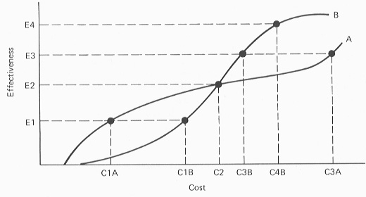
The objective of a cost-goal study is to develop a cost curve for each program alternative. This curve approximates the sensitivity of costs (inputs) to changes in the level of goal achievement (outputs). Costs may change in direct proportion to the level of achievement; that is, each additional increment of cost may produce the same increase in output. However, if output increases more rapidly than costs, then the program alternative is operating at a level of increasing return. This condition is represented by a positively sloped curve that rises at an accelerating rate, as illustrated by the initial segment of cost curve B in Exhibit 6. If costs increase more rapidly than output, the program alternative is operating in an area of diminishing returns (as in the upper segment of cost curve B).
Exhibit 6. Cost-Effectiveness Analysis in Graphic Form
Cost-effectiveness analysis requires a model that can relate incremental costs to increments in achievement. For some types of problems, practical models can be developed with relative ease. For other problems, cost curves can be approximated from historical data. As the input-output relationships associated with various program alternatives are better understood, the construction of cost curves and effectiveness scales should become increasingly more sophisticated.
Assuming that the costs associated with different achievement levels can be determined for each alternative, the problem remains of how to choose among these alternatives. In principle, the rule of choice should be to select the alternative that yields the greatest excess of positive effects (attainment of objectives) over negative impacts (resources used, costs, and negative spillover effects). In practice, however, this ideal criterion is seldom applied, as there is no practical way to subtract dollars spent from the non-monetary measures of effectiveness.
The best approach, therefore, may be a cost-effectiveness comparison of program alternatives, as illustrated in Exhibit 6. Alternative A achieves the first level of output (O1) at a relatively modest level of cost (C1A), whereas nearly twice the amount of resources (C1B) would be required to achieve the same level of effectiveness using alternative B. Both alternatives achieve the second level of output (O2) at the same level of cost (C2). Alternative B requires a lower level of resources (C3B) to achieve the third level of output (O3). And only alternative B achieves the fourth level of output (O4), since the program cost curve of alternative A is not projected to reach this level of effectiveness.
Significant shifts in the configuration of the cost curves frequently occur in the formulation of program alternatives as additional levels of effectiveness are sought. Thus, program A may provide the most desirable ratio at one level of effectiveness (and cost), whereas at a higher level of effectiveness (and cost), some other program may provide the more desirable ratio.
Which of the two program alternatives is more desirable? To answer that question, it is necessary to define the optimum envelope formed by these two cost curves. If resources in excess of C2 are available, then alternative B is clearly the better choice. However, if available resources are less than C2, alternative A provides greater effectiveness for the dollars expended.
In general, it may not be possible to choose between two alternatives simply on the basis of cost-effectiveness unless one alternative dominates at all levels of goal achievement. Usually, either a desired level of performance must be specified and then costs minimized for that effectiveness level, or a cost limit must be specified and achievement maximized for that level of resource allocation.
In practice, organizations may adopt programs that are do not the most effective technically available. Among the more obvious reasons for this are legal constraints, technical capacity, employee rights, union rules, and community attitudes. The purpose of a cost-constraint assessment is to examine the impact of these factors by comparing the cost of the program that might be adopted if no constraints were present with the cost of the constrained program.
This analysis, shown graphically in Exhibit 7, starts with the expressed goal O1 and two programs (P constrained and P not-constrained). P not-constrained represents the most effective program as determined by cost-effectiveness analysis. The constrained program, however, may be the only program available. The cost of the constraints to the agency is the difference between the program cost of P constrained and P not- constrained
Exhibit 7. Cost-Constraint Analysis in Graphic Form
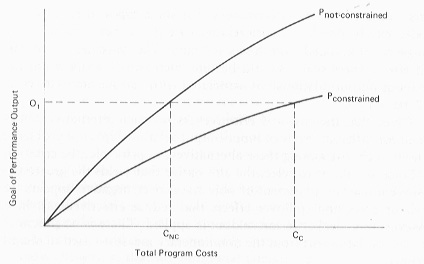
Once this cost differential has been identified, decisions can be made as to the feasibility of eliminating the constraints. This assessment gives decision makers an estimate of how much would be saved by the relaxation of a given constraint. By the same token, the cost of the constraint suggests of the amount of resources that might be committed to overcoming it. In some cases, however, maintaining a constraint may be more important for social or political reasons than implementing a more effective program.
It is now possible to examine how costs and benefits (program effectiveness) are related in the tests for preferredness. Since decision-makers do not know the level of training that can be supported given limited resources, it is necessary to develop a schedule of costs and benefits over the full range of workers to be trained each year (i.e., 0 to 3,000). Program A would require 10 training centers for 3,000 trainees and program B would require 15 centers. The development, investment, and ten years of operating costs are summarized in Exhibit 10 for various levels of coverage.
Based on these data, it is possible to identify the best program given either a fixed budget or a specified level of benefits. Program B is preferred for all budgets under $32.5 million because it would have a greater trainee capacity. Conversely, for all trainee loads less than 1,800, Program B is preferred because it will cost less than Program A. For budgets above $32.5 million or trainee loads above 1,800, Program B is preferred. For example, at a budget of $26 million, Program A has an annual capacity of 1,200 trainees, but Program B could accommodate 1,400 trainees each year for $25.5 million. However, if the objective is to handle an annual training load of 2,400, then Program A would cost $39 million, whereas Program B would cost $43 million. This brief example illustrates how fixed costs (i.e., R&D costs), investment costs (per center), and variable costs (operating costs) can impact the overall cost configuration in different ways.