Unsteady-state modeling of a tubular reactor

 

This is a guide to unsteady-state modeling of PFR-reactors with radial effects using the COMSOL Multiphysics software. The example models a nonisothermal reactor with a nonisothermal cooling jacket.  The reaction is reversible, exothermic, and of 2^nd order

 

A + B2 C

 

which reacts in a tubular reactor (liquid phase, laminar flow regime), same as previous web module on radial heat effects. The reactants are solved in water.

 

The time dependency will be shown as animations of the concentration of species A and the temperature modeled in COMSOL Multiphysics. As shown in Figure 1 the reactants are preheated separately and mixed before entering the reactor. When the start-up begins it takes some time before the preheaters get warmed up, so the inlet temperature of the reaction mixture will increase until it reaches the desired value, T0, which is 320 K. At t=0 there are only solvent in the reactor.

 

 

Model Description

 

 

 

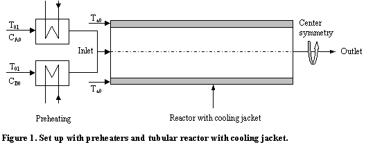
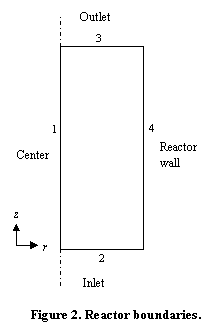
When the reactor is modeled in COMSOL Multiphysics it is assumed that the variations in angular direction around the central axis are negligible, and therefore the model can be axial-symmetric. The system is described by a set of differential equations on a 2D surface that represents a cross section of the tubular reactor in the z-r plane. That 2D surface's borders represent the inlet, the outlet, the reactor wall, and the center line. Due to rotational symmetry, the software needs only to solve these equations for half of the domain shown in Figure 2.

 

Model Equations

The mass balances and heat balances in the reactors are described with partial differential equations (PDEs), while one ordinary differential equation (ODE) is required for the heat balance in the cooling jacket. For the three species A, B and C (all equally expressed and denoted as i) the equations and boundary conditions are defined as follows.

Mass Balance:

where D_p denotes the diffusion coefficient, C_i is the concentration of species i, U is the flow velocity, R gives the radius of the reactor, and r_i is the reaction rate. See the derivation of the mass balance.

Boundary Conditions for the Mass Balance:

1. Center (symmetry) line     2. Inlet (z = 0)       For species A and B an inbuilt heavy side function is used to smoothen the discontinuity between the initial and the boundary concentration. To learn more about this click here.

3. Outlet (z = L) The boundary condition selected for the outlet does not set any restrictions except that convection dominates transport out of the reactor. Thus this condition keeps the outlet boundary open and does not set any restrictions on the concentration.   where L denotes the length of the reactor. 4. At the wall (r = R)   where R is the radius of the reactor. This makes sure that no material flow through the reactor wall.

 

Energy Balance inside the Reactor:

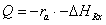
where k denotes the thermal conductivity, T is temperature, r is density, C_p equals the heat capacity, and ΔH_Rx is the reaction enthalpy. To see the derivation of the energy balance, click here.

 

Boundary Conditions for the Energy Balance:

1. Center (symmetry) line

   

2. Inlet (z = 0)

   To use the heat flux as the boundary condition for the inlet the radial effect is included in the uz term and the preheating in T0.
   
   

   
   
   

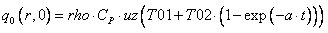
   where q₀ is the heat flux, T01 is the temperature of the reactants before entering the heat exchangers, T02 is the temperature difference between the start temperature (t=0) and the desired inlet temperature, T0. Finally "a" is a heating constant chosen to give a smooth preheating.
   
   

3. Outlet (z = L)

   As for the mass balance, choose the boundary condition at the outlet for the energy balance such that it keeps the outlet boundary open. This condition sets only one restriction, that the heat transport out of the reactor is convective.

    

   
   
   

4. At the wall (r = R)

   

   where T_a denotes the temperature in the cooling jacket.

Energy Balance of the Coolant in the Cooling Jacket:

Here we assume that only axial temperature variations are present in the cooling jacket. This assumption gives a single ODE for the heat balance:

where m_c is the mass flow rate of the coolant, C_Pc represents its heat capacity, and U_k gives the heat-transfer coefficient between the reactor and the cooling jacket. You can neglect the contribution of heat conduction in the cooling jacket and thus assume that heat transport takes place only through convection.

Boundary Condition for the Cooling Jacket:

You can describe the cooling jacket with a 1D line. Therefore you need only an inlet boundary condition.

• Inlet (z = 0)

 

Model Parameters

We now list the model's input data. You define them either as constants or as logical expressions in COMSOL Multiphysics's Option menu. In defining each parameter in COMSOL Multiphysics, for the constant's Name use the left-hand side of the equality in the following list (in the first entry, for example, Diff), and use the value on the right-hand side of the equality (for instance, 1E-9) for the Expression that defines it.

The constants in the model are:

• Diffusivity of all species, Diff = 1E-9 m²/s
• Activation energy, E = 95238 J/mol
• Rate constant, A = 1.1E8 m⁶/(mol·kg·s)
• Gas constant, R = 8.314 J/mol·K (do not confuse this constant with the geometrical extension of the radius)
• Total flow rate, v0 = 5 E-4 m³/s
• Reactant concentrations in the feed, CA0 = CB0 = 500 mol/m³
• Product concentration in the feed, CC0 = 0 mol/m³
• Reactor radius, Ra = 0.1 m
• Catalyst density, r_Cat, rhoCat = 1500 kg/m³
• Heat of reaction, ΔH_Rx, dHrx = -83680 J/mol
• Equilibrium constant at 303 degrees K, Keq0 = 1000
• Thermal conductivity of the reaction mixture, ke = 0.559 J/m·s·K
• Average density of the reaction mixture, r, rho = 1000 kg/m³
• Heat capacity of the reaction mixture, Cp = 4180 J/kg·K
• Overall heat-transfer coefficient, Uk = 1300 J/m²·s·K
• Inlet temperature of the coolant, Ta0 = 273 K
• Heat capacity of the coolant, CpJ = 4180 J/kg·K
• Coolant flow rate, mJ = 0.01 kg/s
• Reactant temperature before entering the preheaters, T01 = 273 K
• Temperature difference between T01 and the final inlet temperature, T02 = 47 K
• Preheating constant, a = 0.03 s^-1

Next, the following section lists the definitions for the expressions this model uses. The expressions are stated under Scalar Expression in COMSOL Multiphysics's Option menu. Again, to put each expression in COMSOL Multiphysics form, use the left-hand side of the equality (for instance, u0) for the variable's Name, and use the right-hand side of the equality (for instance, v0/(pi*Ra^2)) for its Expression.

• The superficial flow rate is defined according to the analytical expression

   

  which we define in COMSOL Multiphysics as u0 = v0/(pi*Ra^2).
  
  

• The superficial, laminar flow rate

  

  in COMSOL Multiphysics form becomes uz = 2*u0*(1-(r/Ra).^2).
  
  

• The conversion of species A is given by

  

  which in COMSOL Multiphysics form is xA = (cA0-cA)/cA0.
  
  

• The rate of reaction looks like:

   

  which in COMSOL Multiphysics form is rA = -A*exp(-E/R/T)*rhoCat*(cA.*cB-cC^2/Keq).
  
  

• The temperature-dependent equilibrium constant is given by the following expression:

  

  which in COMSOL Multiphysics form is Keq =Keq0*exp(dHrx/R*(1/303-1/T)).
  
  

• The heat-production term becomes

  

  which in COMSOL Multiphysics form is Q = (-rA)*(-dHrx).
  
  

• The reaction rates of B and C becomes

  

  
  
  

  Which in COMSOL Multiphysics form is rB=rA and rC=-2*rA

After typing this into COMSOL Multiphysics we are now ready to solve. To see a detailed description on how to set up the model click here.