Model Set-Up Guide

The FEMLAB 3.0 and 3.1i files necessary to solve this problem are available below, but the full version of FEMLAB 3.0, FEMLAB 3.1i or COMSOL Multiphysics must already be installed on the computer to use these files. Once you have downloaded these files, go to the Mesh section and follow the instructions.

FEMLAB 3.0

FEMLAB 3.1i

The text which follows shows how these files were generated

1. Model Navigator

To begin your session to construct the COMSOL Multiphysics model from scratch click, on the COMSOL Multiphysics icon. You will now see the Model Navigator where you can select the desired physics for your model.

1.A. Click the New tab and select 2D-symmetry from the Space dimension list.

1.B. Open the Chemical Engineering Module by clicking on the '+' sign.

1.C. Double-click on the submenu Mass Balance and select Convection and Diffusion.

1.D. Below type the name of the variable(s) you wish to use, cA, cB, cC, and the name of the application, which is MassBalance then click on the Multiphysics button and click Add to add the application mode to your model.

1.E. Do the same things for the energy balance, select Convection and Conduction, type the variable name, T, and add the physic to your model, see Figure 1 below.

1.F. To get the non-isothermal cooling jacket a weak-form boundary application is needed. Select 2D in the space dimension list.

1.G. Open the ODE Modes by clicking on the COMSOL Multiphysics folder and select Weak Form Boundary. The dependent variable name for this application could be Ta that is the temperature of the coolant and Application mode name EB_CoolingJacket.

1.H. Click the Add button. Now everything is set to start modeling the reactor we want.

1.I Click OK to confirm and exit the Model Navigator.

 

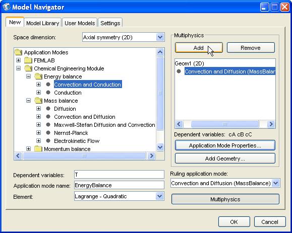
       Figure 1. Adding physics in Model Navigator.

 

2. Options

To let COMSOL Multiphysics know your input data the first thing to do is to define constants and expressions. The Constants dialog box can be found under the Option menu. 2.A. Open the constants window and type in the input data, variable names under Name and the values under Expression, see Figure 2. Click OK.

 

       Figure 2. Entering Constants

 

2.B To add the expression needed select Scalar Expressions under Options menu and Expressions. Here you add rate law expressions, laminar flow expressions etc. For example the conversion expression is typed in as xA= (cA0-cA/cA0), see Figure 3.

 

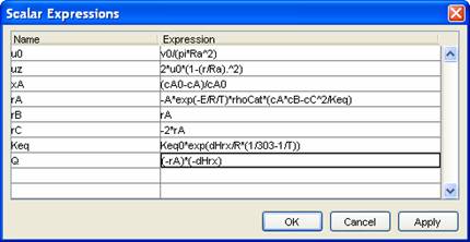
       Figure 3.  Scalar Expression typing.

 

We can now reach the constants and scalar expressions anywhere in COMSOL Multiphysics's edit fields like subdomains and boundaries. Click OK to exit.

 

3. Draw

The structure of a tubular reactor is drawn in COMSOL Multiphysics as a two dimensional rectangle in the z-r plane. A rectangle would correspond to the physics we added by showing the cross section of half of the reactor. Since we assume rotational symmetry, which means that any variations in angular direction around the central axis are negligible, this has the advantage that COMSOL Multiphysics only need to solve for half of the reactor.

 

3.A Select Rectangle/Square in Draw Objects in the Draw menu and draw a rectangle by randomly click on two different coordinates in the coordinate system. You have now created an object denoted as R1 by the software.

3.B Double-click on the object and you will get a window to enter data specifications.

3.C Enter the width and length of the reactor (0.1, 1), and select the position of the object in the coordinate system, i.e. Corner, (0,0). Click OK

3.D Select Axis/Grid Settings in the Options menu and clear the Axis equal box on the Axis tab. Type in axis values for r (-0.2, 0.2) and z (-0.1, 1.1). Click OK to exit.

 

4. Physics Mode

To be able to solve the differential equations we need to specify initial values boundary values etc for each physic we have added to the model.

4.A Select the Mass balance in the Multiphysics menu.

4.B Then go to Subdomain Settings in the Physics menu.

4.C Select subdomain 1 and the cA tab, type in variable names for diffusion (Diff), reaction rate(rA), and z-velocity (uz), see Figure 4.

4.D Click on the Artificial diffusion button and select Isotropic diffusion. Click OK.

4.E Click the Init tab and type in initial the value wanted for each species in the reactor at t=0 (In this case 0 for all species).

4.F Do the same for species B amd C. Exit by clicking OK.

 

       Figure 4. Subdomain Settings for mass balance.

 

4.G Go to Boundary Settings in the Physics menu. Here we can choose the condition at all four boundaries of the reactor. 4.H Select boundary 1 and choose Insulation/Symmetry.

4.I Select boundary 2 and choose Concentration and type cA0*flc2hs(t-10,5) to be score that the feed has initial concentration of A.

4.J On boundary 3, select Convective flux (diffusive flux is negligible here)

4.K On boundary 4, select Insulation/Symmetry.

4.L Do the same for species B and C.

4.M Switch to EnergyBalance in the Multiphysics menu and go to subdomain settings.

4.N On subdomain 1, Physics tab, type in the thermal conductivity (ke), density of the reaction mixture (rho), the heat capacity (C_P), heat source (Q) and z-velocity (uz).

4.O On the Init tab type in a value or expression for initial temperature in the reactor, T0.

4.P Go to Boundary condition and select Axial Symmetry on boundary 1.

4.Q On boundary 2 to get the radial effects we choose Heat flux and type in the following expression, rho*Cp*uz*(T01+T02*(1-exp(-a*t))), see Figure 5. The expression for uz makes the flux parabolic and included in parenthesis is the preheating expression.

4.R For boundary 3 select Convective flux

4.S On boundary 4, select Heat flux and type in -Uk*(T-Ta), to get the heat transfer between the reaction mixture and the coolant.

 

       Figure 5. Boundary Settings for energy balance.

 

 

4.T Finally, select the Weak From, Boundary application and go to Boundary condition in the physics menu.

4.U In the Boundary selection list, mark each point 1-3 and click in the Active in this domain box to make them inactive.

4.V Select boundary 4 and type in Ta0 as the initial value under the Init tab. Select the Weak tab and enter "Ta_test*(TaTz-2*pi*Ra*Uk*(T-Ta)/(CpJ*mJ))" in the weak term expression field to define the weak form energy balance of the cooling jacket, see Figure 6. Click OK.

4.X Go to Point Settings- Equation Systems that can be found under Equation Systems in the Physics menu.

4.Y First select point 3 and go to the Init tab and type in initial temperature of the coolant, Ta0.

4.Z After that select the Weak tab at the constr edit field and type in Ta-Ta0 in the fifth position to tell that Ta0 is the initial temperature at point 3, which is the inlet of the coolant. Ta-Ta0 is then an implicit expression that equals to zero. Click the Apply button to view a key-lock on boundary 3 (see Figure 6). Click OK.

 

       Figure 6. Weak Form conditions for cooling jacket.

 

 

 

5. Mesh

FEMLAB 3.1i

5.1.A One way to set a mesh is to use map mesh which is a square net that solves for every intersection between the lines. Go to Map Mesh in the Mesh menu.

5.1.B Select Boundary, click in the Select all box and type in 60 in the Number of edge elements edit field and click on the Remesh button, see Figure 7.

FEMLAB 3.0

5.2.A If you are using FEMLAB 3.0, go to the Mesh menu and click on Initialize mesh.

5.2.B Again go to the Mesh menu and select Refine Mesh You can see how many elements you have in the lower left corner. Refine mesh again until you have 4480 elements. This will take a while to solve. A mesh of 1120 elements will solve quickly but the result will be less smooth. Exit by clicking OK.

 

       Figure 7.  Map Mesh set-up for FEMLAB 3.1i.

 

 

6. Solve

6.A Select Solver Parameters in the Solve menu to open the Solver Parameters dialog box.

6.B Select Time dependent from the Solver list and in the Times edit field type in 0:1:400, which declares that COMSOL Multiphysics solves the model every second up to 400 seconds, see Figure 8.

6.C Press the solve button ("="). Click OK.

 

       Figure 8. Solver Parameters options.

 

 

7. Postprocessing

7.A In the postprocessing menu, which you can find in Plot Parameters under the Postprocessing menu, you can plot and post process your results. The Surface tab shows the cross section of the reactor.

7.B To view the concentration, choose Concentration, cA (MassBalance) in the Predefined quantities field and click OK, see Figure 9.

7.C You can view the concentration at different times by clicking on the General tab and select the desired time in the Solution at time field.

7.D To animate your result select the variable you want to plot under the Surface tab and click the Animate tab.

7.E Here you select time steps by choosing Interpolated time in the Select via field. Type a matrix of the from "start time : length of time step : end time" (i.e. 0:5:400). Then click Start animation.

 

       Figure 9. Plot Parameters options.