Attainable Region Theory

Summary

In the Introduction we wrote the mole balances for the PFR and CSTR in vector notation.

PFR: e.g. d[cA,cB]/dt = [rA(cA,cB),rB(cA,cB)]
CSTR: e.g. [cA,cB]-[cAo,cBo] = [rA(cA,cB),rB(cA,cB)]

We will now write these equations in a general form that can be used for any problem.

The Characteristic Vector

The listed co-ordinates of a point that specify the product of a system is termed the characteristic vector, c. Remember from vector mathematics that the co-ordinates of a point can also be considered as a vector from the origin. The characteristic vector characterises the state (or composition) of a stream.

For our example: c = [cA,cB]

The characteristic vector must contain sufficient variables to fully describe the reaction kinetics. In our system the reaction kinetics only depend on cA and cB, so we only need to include these in the characteristic vector.

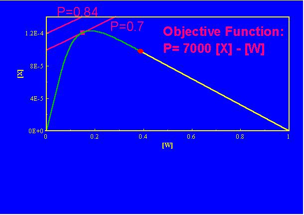
It must also contain sufficient variables to describe the objective function. The objective function is the function that we are trying to optimise. In our case we are trying to maximise the production of B, so the objective function is just:

P = cA.

There are thus no extra variables to add to the concentrations cA and cB to form the characteristic vector. In some problems we may be asked to minimise the total space time of the reactor system. Then we must include the space time in the characteristic vector.

Geometry of the Fundamental Processes

The Reaction Vector and Geometry of Reaction

The vector that contains the rates of formation of the components and thus the kinetics of all the reactions is called the reaction vector, r(c). The reaction vector gives the instantaneous change in state if a mixture of state c undergoes batch reaction. As the equations for a batch reactor are equivalent to the equations for a PFR, the reaction vector also gives the change in the state down the length of a PFR.

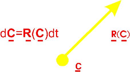
In our example the reaction vector is given by:

r(c) = [rA(cA,cB),rB(cA,cB)] = [-k1cA+k2cB-k4cA^2, k1cA-k2cB-k3cB]
for c = [cA,cB]

The Mixing Vector and Geometry of Mixing

The only other process that may occur in our system is mixing. Mixing can occur in two modes, on its own or within a reactor (for example in a CSTR). Mixing on its own represents the combinig of two process streams to form a single process stream.

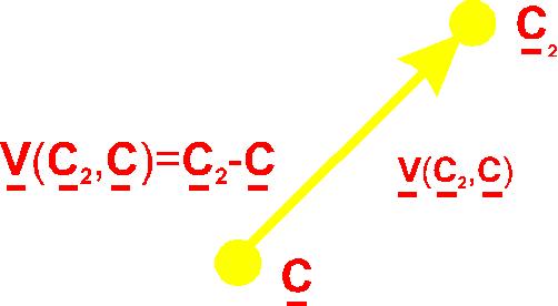
Just as with reaction, mixing is represented by a vector. The mixing vector, v(c₁, c₂), points from the stream being considered to the stream that we are mixing with.

Proof for the mixing vector.

Now that we know the geometry of the fundamental processes let's look at the geometry of some ideal reactors.

Geometry of Ideal Reactors

Geometry of the PFR

We now write the mole balances for the PFR in vector notation as:

dc/dt = r(c)

This means that the reaction vector is tangent to the PFR curve at all points along the PFR curve. This is because of the properties of ordinary differential equation. Because the reaction vector is always tangent the PFR curve is termed a trajectory. Different feed points will lead to different trajectories. The trajectories will never cross because there is only one reaction vector at a point.

PFR Geometry

Geometry of the CSTR

From our previous work we see that we can write the mole balances for the CSTR in our general vector notation as:

c - c⁰ = r(c)t

The general interpretation is that the reaction vector points in the same direction as the mixing vector v=c-c⁰. That is the vectors are colinear. Also the scaled vector r(c)t has the same length as the mixing vector.

CSTR Geometry

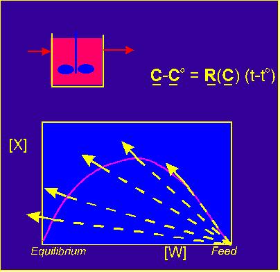
This is true for all the CSTR points, each with a different space time t.

Now that we understand the geometry of the processes and the ideal reactors we can begin to solve problems using the Attainable Region method.

The Attainable Region Method

The Attainable Region is defined as the set of all possible products that can be obtained in a steady-state reactor system with given feed.

There are two reasons that we must find all the possible products:

If our objective function is complicated we do not know where the optimum will occur.
One of the products may be an intermediate that is required to produce the optimum. We will not know what the global optimum is until we have found all the possible intermediate products.

To find the attainable region (AR) requires an iterative construction process. However, we have a set of necessary conditions or "rules" that let us check to see if we have found all the possible products and to help us construct the region.

The necessary conditions that must be satisfied in order for the proposed region to be the AR are:

Constructing the Region

The AR is then constructed by first finding the PFR and CSTR curves starting from the process feed. The necessary conditions are then checked to find any extensions to the region. The necessary condition that is not satisfied will determine how the region must be extended. This process is repeated until all of the necessary conditions are satisfied and there are no further extensions possible. This region is then termed the AR.

Finding the Optimum

Finding the optimum is then the relatively easy procedure of looking for the point on the boundary where the objective function is optimised. This will usually be where one of the lines of constant value for the objective function just touches the boundary of the AR. In this case the objective function will be tangent to the boundary where is touches. Then, from knowing the processes that are required to reach the optimal point, the optimal flowsheet can be determined.

Finding the Optimal System