COMSOL ECRE Instructions

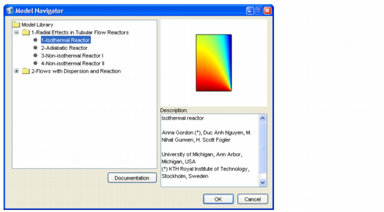
The model presented in this section gives a brief introduction on the use of the COMSOL ECRE Version. This model treats an isothermal tubular reactor with an elementary 2nd-order reversible reaction (liquid phase, laminar flow regime).

The isothermal tubular reactor deals with composition variations in both the radial and axial directions. The section below provides a general description of the model.

More models can be found on the COMSOL ECRE CD including heat transfer effects, both by considering a heat of reaction and by the addition of a cooling jacket.

Model Description

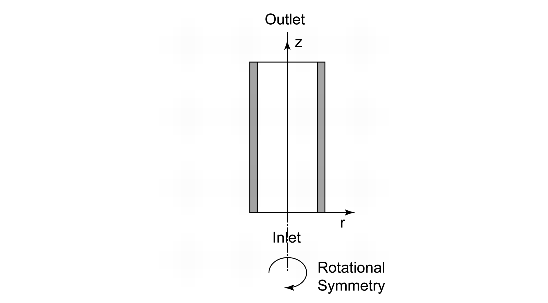
Figure 1 illustrates the model geometry. We assume that the variations in angular direction around the central axis are negligible, and therefore the model can be axi-symmetric.

The system is described by a partial differential equation on a 2D surface that represents a cross section of the tubular reactor in the z-r plane. That 2D surface’s borders represent the inlet, the outlet, the reactor wall, and the center line. Assuming that the diffusivity for the three species is of the same magnitude, you can model the reactor using one mass balance for one of the species (as noted in the next section, mass balances are not necessary for the other two species). Due to rotational symmetry, the software need only solve this equation for half of the domain shown in Figure 1.

Model Equations for the Isothermal Tubular Reactor

You describe the mass balance in the reactor with a partial differential equation. The equation is defined as follows.

Mass Balance, species A:

where D_p denotes the diffusion coefficient, C_A is the concentration of species A, U is the flow velocity, R gives the radius of the reactor, and r_A is the reaction rate. In this model we assume that the species A, B, and C have the same diffusivity, which implies that we must solve only one material balance; we know the other species’ concentrations through stoichiometry.

Boundary Conditions for the Mass Balance:

• Inlet (z = 0)

• At the wall (r = R)

• Center (symmetry) line

The boundary condition selected for the outlet does not set any restrictions except that convection dominates transport out of the reactor. Thus this condition keeps the outlet boundary open and does not set any restrictions on the concentration.

• Outlet (z = L)

where L denotes the length of the reactor.

Model Parameters

We now list the model’s input data. You define them either as constants or as logical expressions in COMSOL Multiphysics’s Option menu. In defining each parameter in COMSOL Multiphysics, for the constant’s Name use the left-hand side of the equality in the following list (in the first entry, for example, Diff), and use the value on the right-hand side of the equality (for instance, 1E-9) for the Expression that defines it.

The constants in the model are:

• Diffusivity of all species, Diff = 1E-9 m²/s
• Activation energy, E = 95238 J/mol
• Rate constant, A = 1.1E8 m⁶/(mol�kg�s)
• Gas constant, R = 8.314 J/mol�K (do not confuse this constant with the geometrical extension of the radius)
• Inlet temperature, T0 = 320 K
• Total flow rate, v0 = 5 E-4 m³/s
• Reactant concentrations in the feed, CA0 = CB0 = 500 mol/m³
• Reactor radius, Ra = 0.1 m
• Catalyst density, _Cat, rhoCat = 1500 kg/m³
• Equilibrium constant at 303 degrees K, Keq0 = 1000

Next, the following section lists the definitions for the expressions this model uses. Again, to put each expression in COMSOL Multiphysics form, use the left-hand side of the equality (for instance, u0) for the variable’s Name, and use the right-hand side of the equality (for instance, v0/(pi*Ra^2)) for its Expression.

• The superficial flow rate is defined according to the analytical expression

which we define in COMSOL Multiphysics as u0 = v0/(pi*Ra^2).

• The superficial, laminar flow rate

in COMSOL Multiphysics form becomes uz = 2*u0*(1-(r/Ra).^2).

• The conversion of species A is given by

which in COMSOL Multiphysics form is xA = (cA0-cA)/cA0.

• The concentration of B is according to

which in COMSOL Multiphysics form becomes cB = cB0-cA0*xA.

• The concentration of C is expressed as

which in COMSOL Multiphysics form becomes cC = 2*cA0*xA.

• The rate of reaction takes two forms:
• For the isothermal reactor, the reaction rate looks like

,

which in COMSOL Multiphysics form is rA = -A*exp(-E/R/T0)*rhoCat*(cA*cB-cC^2/Keq).

• The temperature-dependent equilibrium constant is given by the following expression for the isothermal case:

which in COMSOL Multiphysics form is Keq = Keq0*exp(dHrx/R*(1/303-1/T0)).

Reviewing the Model in the COMSOL ECRE Version

Opening the Model

1. Insert the COMSOL ECRE CD and select the platform on which you wish to run it. The Model Navigator window then appears on the screen.
2. In this window click the folder 1-Radial Effects in Tubular Flow Reactors, and then select the model 1-Isothermal Reactor. Click OK.
   
   

   The model opens in Postprocessing mode, and the surface plot shows the concentration of species A in the reactor.

   

   Note that the plot does not display the reactor’s dimensions with equal axes in the r- and z-directions.

Model Equations and Input Data

In COMSOL ECRE you can review and change the model equations and input data, but you cannot add or remove the so-called application modes that implement the model. To review the application modes the model makes use of, do the following:

1. Click the Multiphysics menu. Doing so opens a drop-down list that contains any active application modes, in this case the Convection and Diffusion (Mass Balance) application mode.
2. Click on the Multiphysics menu again to close the list.
3. Go to the Physics menu and select Subdomain Settings, which opens up the corresponding dialog box. Select subdomain 1 in the Subdomain Settings list. This dialog box displays the equation that forms the basis for this application mode, while the edit fields show the input data used in the equation.
   
   
4. The edit fields correspond to the diffusion coefficient, reaction-rate expression, and velocity distribution in the reactor—all of which you can freely define. To review and change the definition of the input data, follow this procedure:
5. Go to the Options menu and select Constants. The resulting dialog box displays the names and definitions of all the constants used in the model.
   
   
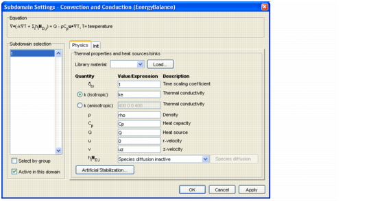
6. You can freely define new constants and rename existing ones. In the dialog box in the preceding figure you can identify Diff, which is the diffusion coefficient entered in the Diffusion coefficient edit field in the Subdomain Settings dialog box. COMSOL ECRE also allows for the definition of expressions.
7. Go to the Options menu, then to the expandable menu item Expressions, and finally select Scalar Expressions.
   
   
8. It is possible to move the Scalar Expressions dialog box in order to also display the Constants dialog box. Look closely at the definitions of the scalar expressions and recognize that they use constants from the Constants box. Note also that the constants and the scalar expressions are defined according to the list of Model Parameters in the preceding section. Examine the Subdomain Settings box and note that the scalar expression rA in the Reaction rate edit field defines that parameter, and the scalar expression uz in the z-velocity edit field defines the corresponding velocity component.
9. Click the Cancel button in both the Scalar Expressions, Constants, and Subdomain Settings dialog boxes.
11. Having reviewed the domain equations in the model, you can proceed to the boundary conditions.
12. Go to the Physics menu and select Boundary Settings.
13. Click on boundary number 1 in the Boundary Selection list. It corresponds to the reactor’s central axis.
    
    
14. Select boundary number 2 to view the boundary condition at the reactor’s inlet. In this case, the constant cA0 defines the inlet concentration in the Boundary Condition of type Concentration. You can find the constant’s value in the Constants dialog box under the Options menu.
15. Select boundary number 3 to review the outlet boundary condition, which in this case is a Convective flux condition. You can use this condition when it is safe to assume that the transport of mass perpendicular to the outlet is dominated by convection. The boundary condition sets the diffusion term in the mass-flux vector in the outlet direction to zero.
16. Select boundary number 4 to review the last condition, which corresponds to the reactor’s outer wall and is therefore an insulating boundary for the mass balance.
17. Click the Cancel button to close the Boundary Settings dialog box.

You have now reviewed the input data, domain equations, and boundary conditions. To repeat, while you can change all these definitions, you cannot replace or expand the Convection Diffusion application mode when running COMSOL ECRE; you need the full COMSOL Multiphysics Chemical Engineering Module to extend the model to include, for example, additional mass balances.

Visualizing the mesh

Further, while you cannot manipulate the mesh in COMSOL ECRE, it does allow you to visualize the mesh by pressing the Mesh Mode button.

Note in this case that the scales on the r- and z-axes are not equal, which gives a distorted view. If desired, you can select equal scale settings in the Axis/Grid Settings menu item under the Options menu. In order to return to the original unequal scale settings, once again go to the Axes/Grid Settings menu and clear the Axis equal check box. Enter -0.1 in the r min edit field, 0.2 in the r max edit field and -0.1 and 1.1 in the z min and z max edit fields, respectively.

Checking the Solver Settings

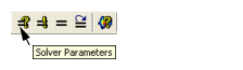
COMSOL ECRE allows you to change the equation parameters and reaction kinetics and then solve the problem again. The model in this exercise is nonlinear; thus press the Solver Parameters and verify that the Stationary nonlinear solver is selected.

Postprocessing

COMSOL ECRE comes with the full set of COMSOL Multiphysics postprocessing capabilities. These include surface plots, cross-sectional plots, point plots, as well as boundary and subdomain integrations. Now is a good time to review some of the software’s plotting and postprocessing capabilities.

1. Click the Postprocessing Mode button. The default plot shows the concentration of species A in the reactor.
   
   
   
   
2. Click the Plot Parameters button.
   
   
3. Click on the Surface tab.
4. On the Surface page, enter -rA in the Expression edit field.
   
   
5. Click Apply.
   
   
6. To plot the conversion of species A, enter xA in the Expression edit field in the Plot Parameters dialog box.
7. Click Apply.
   
   
8. In order to define the location of the maximum and minimum conversion, click the Max/Min tab.
9. Enter xA in the Expression edit field in the Subdomain max/min data dialog box.
10. Click the Max/min marker check box and click Apply.
11. To visualize the relation between residence time and conversion, first click the Max/min marker check box to deselect it and click the Arrow tab in the Postprocessing menu.
12. Select Total flux,cA in the Predefined quantities drop-down list.
13. Click the Arrow plot check box and click OK.
    
    
14. To visualize the local conversion in selected cross sections along the length of the reactor, first go to the Postprocessing menu and select Cross-Section Plot Parameters.
15. Click the Line/Extrusion tab.
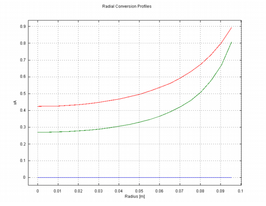
16. Enter xA in the Expression edit field.
17. Enter 0 in the r0 edit field and 0.1 in the r1 edit field.
18. Enter 0 in both the z0 and z1 edit fields.
19. Check the Multi parallel lines box, then click the Vector with distances option.
20. Enter 0 0.5 1 in the Vector with distances edit field to generate three cross-section plots at the inlet, in the middle of the reactor, and at the outlet, respectively.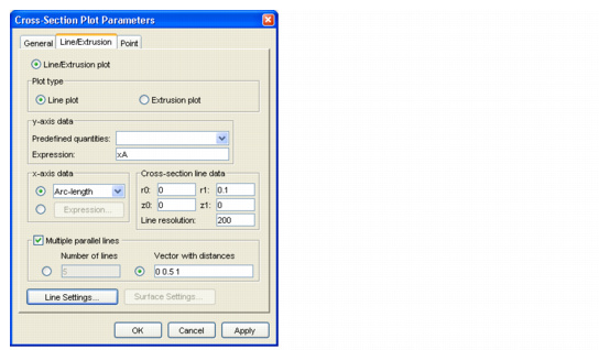
    
    
21. Click the Line Settings button. In the dialog box that opens, select the Cycle option in the Line color drop-down list; select Dotted line in the Line style drop-down list; and select Cycle in the Line marker drop-down list.
    
    
22. Finally, to generate the following plot, click OK twice: first in the Line Settings dialog box, and then in the Cross-Section Plot Parameters dialog box.
    
    
    Figure 2: Radial conversion profiles at the inlet, outlet and halfway through an isothermal reactor.
    
    
23. COMSOL ECRE can also calculate integral expressions of the solution. One such entity is the mixing cup outlet concentration, which gives the average concentration in the liquid that exits the reactor. For species A, the average concentration is defined according to the equation
    

    along the outlet boundary. Start by calculating the integral of C_Au_z over the outlet boundary.
24. Go to the Postprocessing menu and select Boundary Integration.
25. Select boundary 3 in the Boundary selection list.
26. Enter 2*pi*r*cA*uz in the Expression edit field.
27. Click Apply.
28. The value of the integral appears in the status bar at the bottom and reads 0.114385. You can now calculate the integral of u_z.
29. Enter 2*pi*r*uz in the Expression edit field and click Apply.
30. The value of this integral is 5e-4, which gives an average concentration of 0.114385/5e-4, which is approximately 230 mole m^-3.

You have now completed a review of the Isothermal Tubular Reactor model. More models and corresponing excercises can be found on the COMSOL ECRE CD.