COMSOL Multiphysics is a modeling package that solves arbitrary systems of partial differential equations (PDEs). It allows you to solve these equations in two ways: First, in what we refer to as PDE modes, you enter the equations from scratch at the keyboard. Second, the software provides a far easier method of solving commonly encountered equations whereby you take advantage of ready-made application modes targeted at the problem areas the equations describe. For example, the Navier-Stokes application mode implements a predefined interface for the modeling of laminar flow as described by the Navier-Stokes equations.
The Chemical Engineering Module that comes as an add-on to COMSOL Multiphysics delivers a selection of these ready-made application modes for transport and reaction processes found in chemical engineering. That module was inspired by two classic chemical-engineering texts: Fogler’s Elements of Chemical Reaction Engineering and Bird, Stewart, and Lightfoot’s Transport Phenomena.
The Chemical Engineering Module is divided into three application mode menu trees:
All application modes in COMSOL Multiphysics are equation-based. This means that by selecting a ready-made application mode you can easily modify or extend the built-in equations. For example, you might elect to enter expressions for source and sink terms such as reaction terms.
The following sections offer a short presentation of the application modes in the Chemical Engineering Module.
The momentum balances application modes encompass the relevant equations for a large variety of fluid-flow applications.
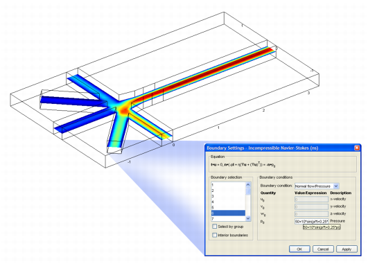
Incompressible Navier-Stokes: This application mode defines and solves the Navier-Stokes equations where density is a constant, and it includes a range of possible boundary conditions. You can easily extend it to include driving forces from other phenomena such as electric fields in electrokinetic flow.
Figure 1 shows the flow profile at the junction of several micro-channels, where the inlet velocities at the star-like entrance vary in a sinusoidal fashion. You create these varying flow profiles by specifying a sinusoidal expression for the inlet pressures and introducing a phase shift among the different inlets.
Non-Newtonian Flow: This application mode includes two predefined models for non-Newtonian fluids—the Carreau model and the power law model, which together cover a large group of non-Newtonian fluids. The modeling interface and boundary conditions are similar to those for the general Navier-Stokes application mode.
Non-Isothermal Flow: This is also a version of the Navier-Stokes application mode but allows for density to include temperature dependencies.
k-![]() Turbulence Model: This application mode solves the k-
Turbulence Model: This application mode solves the k-![]() model equations for turbulent flow. It includes logarithmic wall laws and other boundary conditions needed for the simulation of turbulent flow with these equations.
model equations for turbulent flow. It includes logarithmic wall laws and other boundary conditions needed for the simulation of turbulent flow with these equations.
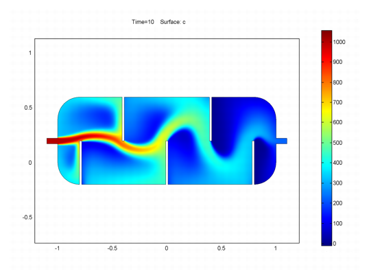
Figure 2 illustrates results from a model of a baffled reactor solved with the k-![]() Turbulence Model application mode. The graph shows the concentration distribution ten seconds after injection at the inlet. The mixing improves with the number of baffles that follow the inlet.
Turbulence Model application mode. The graph shows the concentration distribution ten seconds after injection at the inlet. The mixing improves with the number of baffles that follow the inlet.
Darcy’s Law: This application mode deals with porous media flow as described by Darcy’s law in combination with the continuity equation.
Brinkman Equations: This extension of Darcy’s law includes the influence of viscosity in porous media flow. With it you can treat highly porous structures or combinations of open channels and porous structures such as monolithic reactors.
Euler Flow: This application mode is suitable for the modeling of trans-sonic inviscid flow. It solves the momentum, mass, and energy balances needed to model compressible flow, handling the effects of work done by fluid compression and expansion.
The energy balances application modes account for the transport of energy in fluids and solids as well as the generation of heat through chemical reactions.
Conduction: This application mode defines and solves heat-transfer problems where flux is dominated by conduction. It also includes arbitrary reaction terms where you can define heat generation from reactions.
Convection and Conduction: This application mode couples fluid flow with energy transport. It includes heat transport by conduction, convection, and species diffusion in a solution. In the source term it can incorporate arbitrary expressions for heat generation such as chemical reactions.
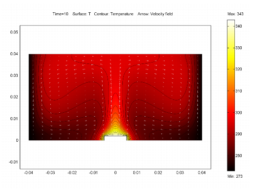
Figure 3 shows the temperature field in an enclosure where a heat source sits at its bottom and the vertical walls are being cooled. The model combines two application modes: Convection and Conduction, and Non-Isothermal Flow. The temperature and density variations induce buoyancy-driven flow in the cavity.
The mass balances application modes deal with a mass balance for each component in the system. They can handle arbitrary expressions for reaction kinetics or other source or sink terms such as phase transfer.
Diffusion: This application mode defines and solves Fick’s law for diffusion in combination with the continuity equation for each species in a solution. You can also include reaction terms.
Diffusion and Convection: This application mode models the transport and reaction of species in dilute solutions. The diffusivity can be an arbitrary function of concentration or temperature, while the convective term can be easily coupled to fluid flow. Alternatively, you can enter independent expressions for convection.
Maxwell-Stefan: This application mode models concentrated solutions where the species in solution interact with each other as well as the solvent. It can also include reactions.
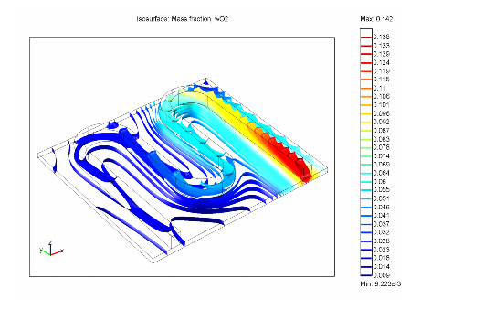
Figure 4 shows the oxygen iso-concentration surfaces in a gas-diffusion cathode for a fuel cell. The model couples the Maxwell-Stefan application mode to the Navier-Stokes application mode, which describes flow in the channels of the current collector.
Nernst-Planck: This application mode defines and solves mass balances where the model considers the transport of charged species in an electric field in addition to the diffusion and convective transport mechanisms. It serves to study electrokinetic transport in electrochemical cells and other devices where ions are subjected to electric fields.