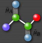
The basic idea of multidimsional spectroscopy is that we can observe the coupling between transitions in condensed phase molecules. The coupling is highly dependent on distance and angles so we can determine structural information. Since the laser pulses we use are all less than ~150 fs, we can measure structrual evolution on sub-picosecond timescales.

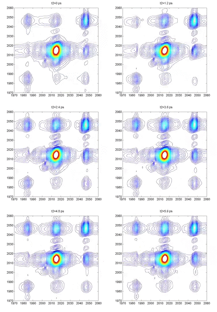
This movie shows several 2DIR spectra of dimanganese decacarbonyl in cyclohexane. The excitation axis is the horizontal, and the detection is on the vertical. The frames are taken at 100 fs intervals, and we can clearly see coherent oscillations in the molecule through the modulations of the cross-peak amplitudes.

Multidimensional Spectroscopy

There are many different ways to study the properties of molecules. Optical spectroscopy has proven to be one of the most useful and general approaches, and it is what we use in our lab. A typical spectroscopic measurement involves measuring how a sample changes the transmission of a light beam (could be a laser or not). The absorption spectrum shows us how a sample absorbs as a function of frequency (or wavelength). These spectra are linear and one-dimensional because they are caused by only very weak interactions with the input light and because they depend on only one frequency, respectively.

While ubiquitous and certainly very useful, traditional linear spectroscopy is incapable of distinguishing, for example, whether two spectral features arise from transitions on the same molecule, or from different molecules within a mixture. Even with only a single chemical species, 1D spectroscopy can say nothing about whether two transitions are close together or far apart in space. These embarrassing ambiguities of one-dimensional spectroscopy can be overcome using multidimensional spectroscopy (MuDSy) where cross-peaks in the 2D spectrum directly map to couplings that are highly dependent on distance and angular orientation. MuDSy techniques are both nonlinear and at least two-dimensional. The following will motivate and introduce MuDSy in general and Fourier transform approaches in particular.

Each 2D spectrum in the animation to the left was recorded in under ten seconds using our new upconversion-based detection method. Here we convert the IR signal into the visible so that we can measure it using a conventional silicon CCD camera. The molecule we studied was a metal cabonyl complex, Mn₂(CO)₁₀, which has many carbonyl units that are all coupled together. The oscillations are due to quantum mechanical superpositions of different vibrational states.

Two Ways to Tune a Bell

Suppose you want to know the resonance frequencies of a bell, how would you measure them? Here's one way: connect a loudspeaker (like the one in your stereo) to a voltage supply, and to that voltage supply, attach a frequency generator that can modulate the output of the voltage generator. Make a physical contact between the vibrating part of the loudspeaker and the bell. Now you can dial a given frequency on your frequency generator and a modulated voltage signal will drive the loudspeaker/bell composite at that frequency. At any given frequency, the bell may or may not be driven due to its particular resonances—if the frequency is one of those at which the bell can vibrate, it will, otherwise it will just sit there. So now you just need to measure what's happening with the bell. When the driver is in resonance with the bell, the bell will vibrate and emit sound. Now listen with something like a microphone—if the bell is vibrating, you know you've hit a resonance. The time-integrated sound amplitude at that driving frequency is one point on your spectrum, now you just need to scan the frequency and repeat until you have fully mapped out the full spectrum.

This isn't the only way to measure the resonance frequencies of the bell, however. Since resonant frequencies are really just all the possible mechanical deformations of the bell's structure, we could arrange to have all those deformations occur at the same time and try to get the frequencies out of the total sound that is emitted. It turns out that there is a very elegant manner in which to proceed: whack the darn bell! By whacking the bell, we excite all (or at least most of) the modes of vibration at the same time. The emitted sound we measure (now we have to measure it as a function of time) contains all the frequencies and we can use the lovely Fourier transform to obtain a spectrum of our bell.

In all forms of spectroscopy, we have precisely the same basic options: sweep a narrowband excitation methodically across the possible frequencies and measure everything that comes out, or deliver an impulsive blow that simultaneously excites all frequencies and Fourier transform the emission. This is what is done in NMR, EPR, FTIR, FT Raman, and even mass spectrometry. The general method is called Fourier transform spectroscopy, and it forms the basis for most recent MuDSy techniques.

Out of Flatland: Beyond 1D Spectra

With the simple bell-tuning picture, it is straightforward to extend spectroscopy to higher dimensions, all we need are more pulses. It turns out that measuring the emission following excitation with two pulses gives you a 2D spectrum, but only if the material is asymmetric (it won't work for molecules in solution, for example). The simplest general case requires three pulses in sequence and the measurement of the electric field emitted by the sample. Since there are then three input “waves” and one output “wave,” the situation is called “four-wave mixing” and is generally done using either infrared or visible pulse sequences to measure the 2D spectra of vibrational or electronic transitions, respectively. The figures on the left describe the method of obtaining a 2D spectrum.

Broadening Mechanisms

What does the multidimensional spectrum tell you? There are basically two key features of a MD spectrum that are qualitatively different from 1D spectra. For the first, let's think about the following problem: you just synthesized a batch of quantum dots and you want to know if they all have the same (or nearly the same) diameter, or whether you have a wide distribution of sizes. You know from simple quantum confinement arguments that the absorption frequency of the dot will depend on its diameter—the larger the dot, the lower the frequency (or longer the wavelength). The emission spectrum will also depend more or less in the same way on diameter, so a small dot will fluoresce blue and large one red. If you mix a bunch of differently sized dots, you will detect a very broad emission profile due to the sum over all the different emission spectra. The only way to know the intrinsic emission is to measure the emission of a single dot, and this is fully within the realm of possibility these days. From your linear, 1D spectrum, however, you can never separate the spectrum due to all the different dots if they overlap spectrally. This is a classic case of an “inhomogeneously” broadened spectrum.

Imagine another situation. You have a dye molecule in a solution, and it has a characteristic fluorescence spectrum, but you happen to know that it is not the same in a different solvent (you might like to reflect on why this might be). Thinking along these lines, however, it is not unreasonable to consider that the environment has an effect on the fluorescence of the molecule. That is to say, for a given solvent configuration and slightly altered dye conformation, you might see different emission. What if the time it takes to interconvert between these microstates is very fast? If it is, we would call the broadening “homogeneous.”

To be sure, inhomogeneous and homogeneous broadening are idealized concepts to begin with and they are extremes to boot! In real life, many systems are not so easily categorized. These two extremes do offer, however, decisive motivation for MuDSy: it is capable of distinguishing these two broadening paradigms, but linear spectroscopy cannot.

Coupling Between Transitions

A spectrum with two or more peaks may result from coupling between different transitions within a molecule. A molecule with two identical transitions (such as two identical carbonyl stretch vibrations) will have only a single peak unless there is some coupling between the two transitions. A simple linear coupling will serve to split the two transitions, and the splitting will reveal the strength of the coupling. There are many examples from atomic physics where line splitting is due to coupling—the Stark effect results from coupling to an external electric field, for example. With the coupling we have another perfectly reasonable way to describe the system: in terms of eigenstates of the “correct” Hamiltonian (i.e. the one with the coupling), in addition to the local mode basis (the uncoupled vibrations). We can say that there are two oscillators coupled together linearly, or that there are two different oscillators (forgetting about their origins as uncoupled oscillators). Since the coupling need not stop at a linear term, we can imagine the more general case of coupling through vibrational anharmonicity of the molecular potential. Thus, learning about how vibrations are coupled together tells us about very interesting terms in the potential above simply those at the harmonic level. Chemistry cannot occur in harmonic molecules since bonds would never break! To learn about chemistry, we must learn about anharmonicity. In general, linear spectroscopy tells us little about anharmonicity, and we can only determine the coupling when there are clearly resolvable spectral lines, and this is rarely the case in interesting condensed phase spectra of complicated molecules.

MuDSy as a Probe of Proteins

In the section on Ultrafast Protein Dynamics, we set out a little recipe for studying protein dynamics through vibrational spectroscopy. Now we tie up the loose ends. The vibrational spectra of proteins are full of information and have been used successfully by all manner of chemists and biologists to characterize proteins. This success is largely due to the secondary-structure-specific Amide I band. There are a lot of clues that indicate that the vibrations are quite well-coupled even at different frequencies, so we will be using multicolor (i.e. two or more) infrared pulse sequences to look at coupling between different kinds of oscillators within proteins, as well as to study what happens following a dramatic triggering event such as a photoisomerization or ligand dissociation.

The key point is that as the protein conformation changes in response to such a trigger, the coupling will also change. Since cross-peak spectra are highly sensitive to the details of the coupling, the 2D spectrum will report directly on the changes of the coupling.

In the longer term, we will combine forces with simulators and theoreticians in order to develop a robust atomic-level understanding of our spectroscopic observables. We will also be developing (alone or in collaboration) modified proteins and protein/ligand combinations to test these models and to explore extremely non-equilibrium conformations (which will include protein folding).

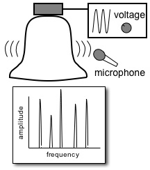
Finding the resonances of a bell by tuning a narrow-band driver. The spectrum is just the integrated amplitude of the bell's emission as deteced with the microphone.

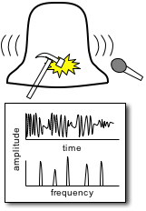
By striking the bell with a hammer and recording the time-domain signal that is emitted by the bell allows us to use Fourier transform techniques. A Fourier transform of the bell sound will reveal the same resonance frequencies as we found with the continuous tuning method.

A series of three pulses is needed to obtain a two-dimensional spectrum. For fixed values of t2, we scan the time delay between the first two pulses, t1, and record the signal's electric field in the frequency domain using a spectrometer giving one frequency axis. Fourier transforming the spectrum with respect to t1 yields the second frequency axis.

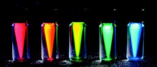
This series of quantum dots—tiny nanoparticles whose energy levels are roughly given by a particle in a sphere description—illustrate an extreme case of inhomogeneous broadening. A mixture of these particles would have a very broad emission spectrum. (image from QuantumDot, Inc.)

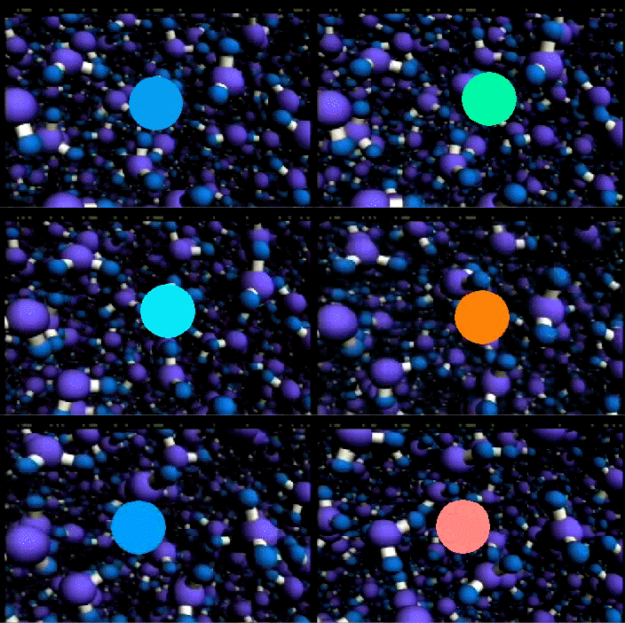
This cartoon animation shows how a dye molecule's transition frequency might change as its environment fluctutates. The animation was made by taking some frames of a molecular dynamics simulation of water by Shinji Saito and Iwao Ohmine.

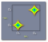
This cartoon two-dimensional spectrum would be observed in the case where there is no coupling between the two transitions. The two transitions may be on two different molecules, or they may be located very far apart within the same molecule.

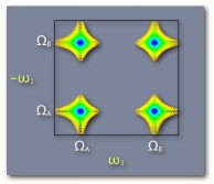
This cartoon 2D spectrum indicates that the transitions are coupled. Excitation at capital omega A leads to emission at capital omega B. The shape of the off-diagonal peak is completely Lorentian and not elongated parallel to the diagonal indicating no inhomogenous broadening. Omega 1 is shown with a minus sign to indicate that the signal shown here is produced in the k2-k1+k3 direction.

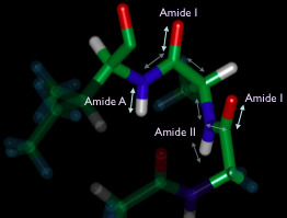
The backbone of a protein (shown above is a turn from an alpha-helix) has several key vibrational transitions that are strongly coupled together and whose frequencies depend on the conformational detail of the larger secondary structure.