Figures
This page contains figures from the book Computational Physics by
Mark Newman. Figures are given in their original resolution-independent EPS
format, and for convenience in PNG image format (useful for including in
presentations). All numbered figures are included here, except the three
figures in Chapter 1, which cannot be distributed for
copyright reasons. You can also download all figures in a single zip file
by clicking here:
There are no figures in Chapters 2, 4, and 11.
Chapter 3: Graphics and visualization
| EPS | PNG | 3.1 | Graph of the sine function
|
| EPS | PNG | 3.2 | Graph of data from a file
|
| EPS | PNG | 3.3a | A basic graph with extra space added
|
| EPS | PNG | 3.3b | A graph with labeled axes
|
| EPS | PNG | 3.3c | A graph with the curve replaced by circular dots
|
| EPS | PNG | 3.3d | Sine and cosine curves on the same graph
|
| EPS | PNG | 3.4 | The Hertzsprung--Russell diagram
|
| EPS | PNG | 3.5 | A example of a density plot
|
| EPS | PNG | 3.6a | Density plot using the default heat map color scheme
|
| EPS | PNG | 3.6b | The gray color scheme
|
| EPS | PNG | 3.6c | The same plot but with different calibration of the axes
|
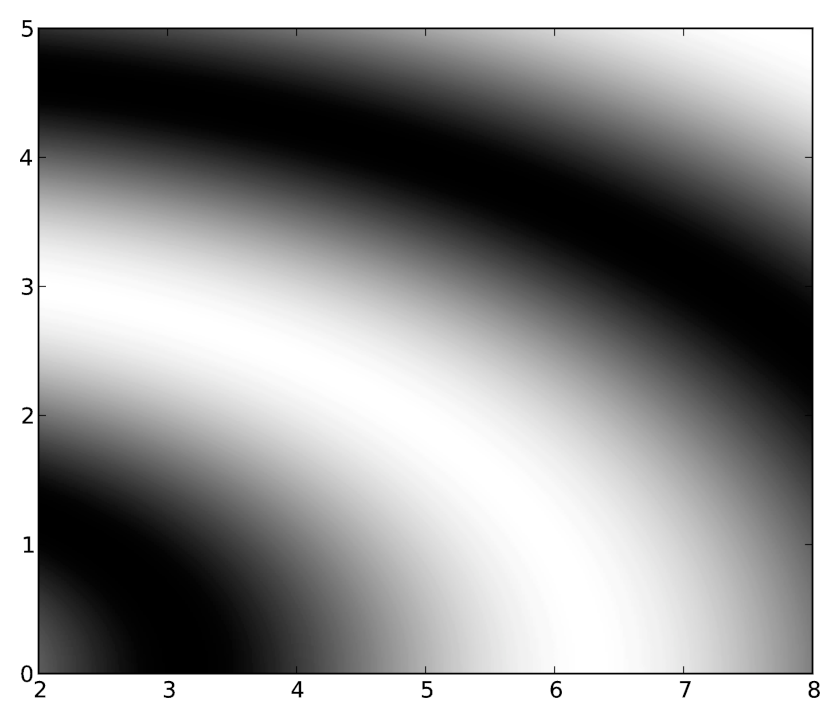
| EPS | PNG | 3.6d | The same plot but with the horizontal range reduced
|
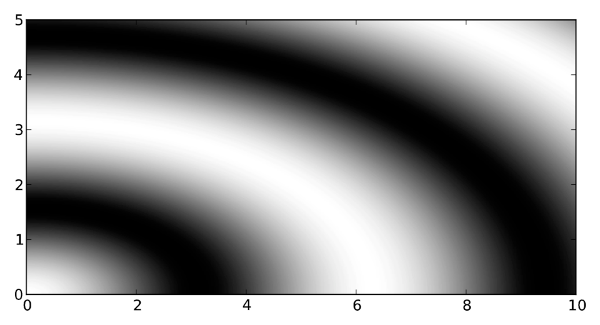
| EPS | PNG | 3.7 | Interference pattern
|
| EPS | PNG | 3.8 | Visualization of atoms in a simple cubic lattice
|
Chapter 5: Integrals and derivatives
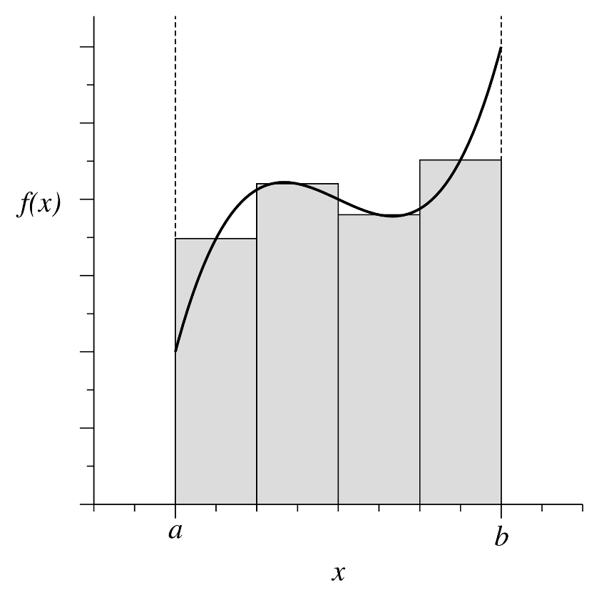
| EPS | PNG | 5.1a | Rectangle rule
|
| EPS | PNG | 5.1b | Trapezoidal rule
|
| EPS | PNG | 5.1c | Trapezoidal rule with more slices
|
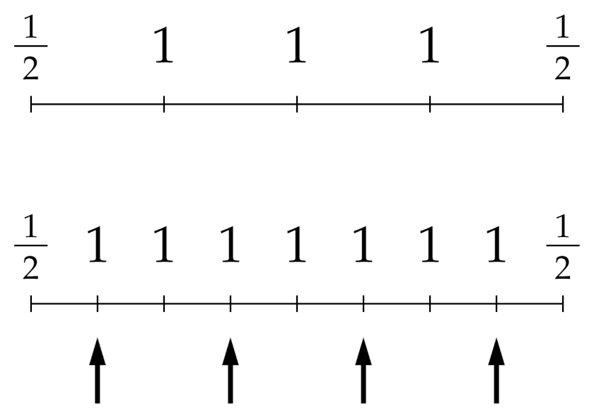
| EPS | PNG | 5.2 | Simpson's rule
|
| EPS | PNG | 5.3 | Doubling the number of steps in the trapezoidal rule
|
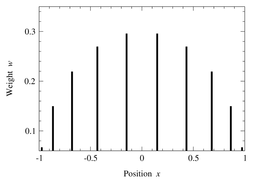
| EPS | PNG | 5.4a | Points and weights for Gaussian quadrature with N = 10
|
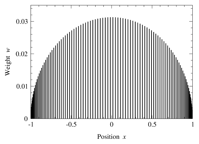
| EPS | PNG | 5.4b | Points and weights for Gaussian quadrature with N = 100
|
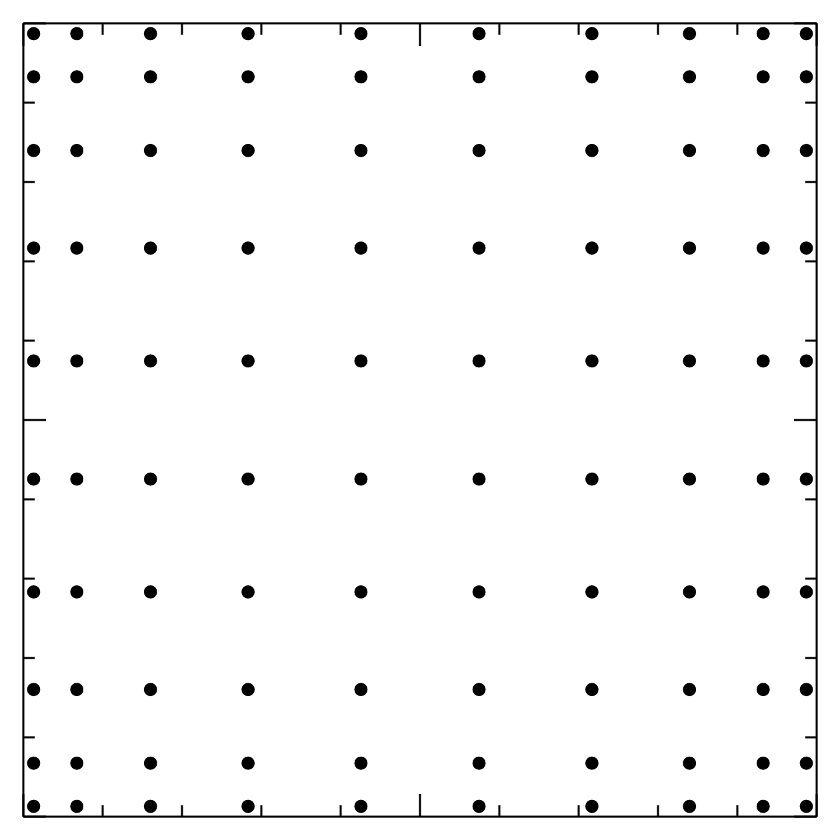
| EPS | PNG | 5.5 | Sample points for Gaussian quadrature in two dimensions
|
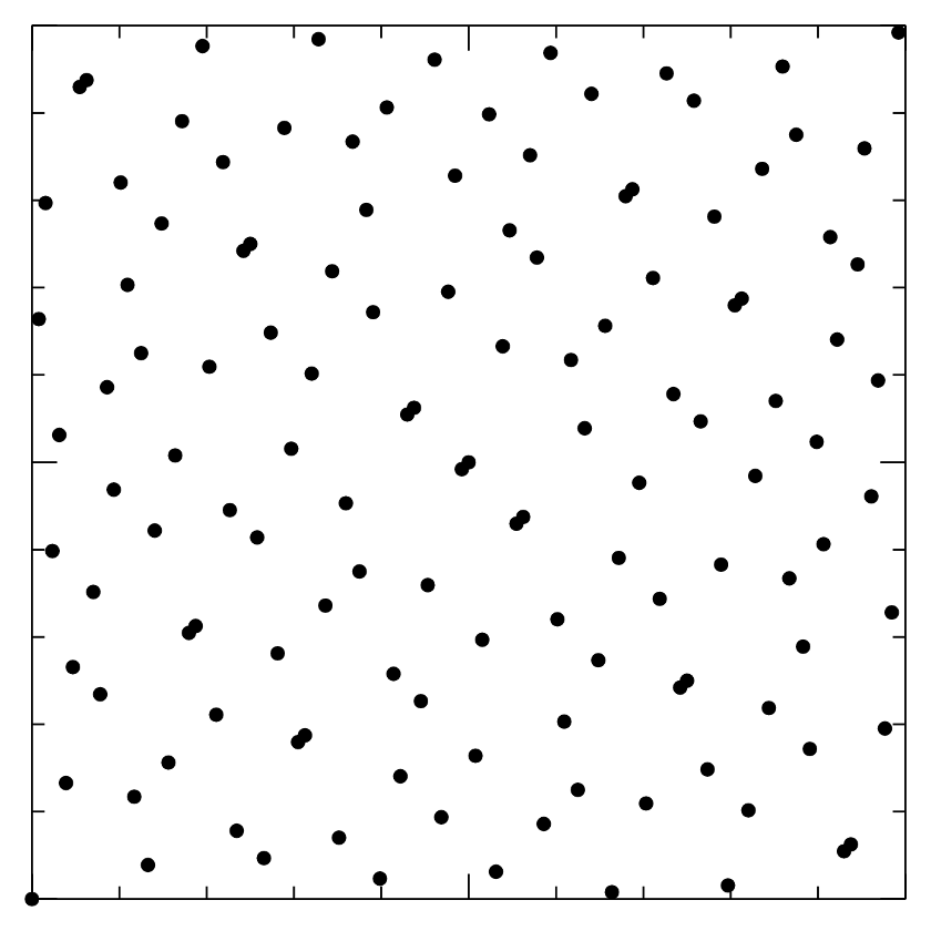
| EPS | PNG | 5.6 | 128-point Sobol sequence
|
| EPS | PNG | 5.7 | Integration over a non-rectangular domain
|
| EPS | PNG | 5.8 | A complicated integration domain
|
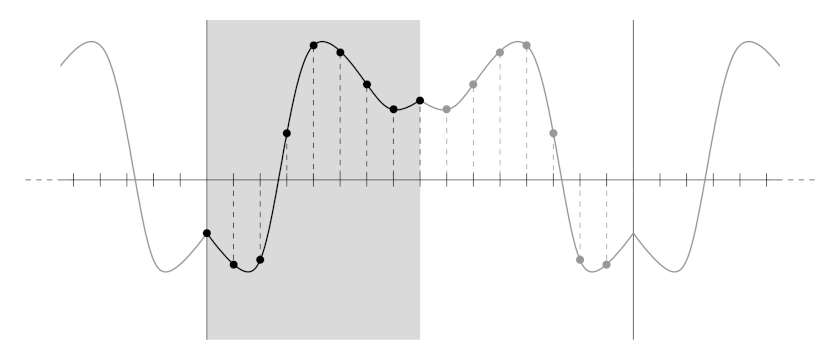
| EPS | PNG | 5.9 | Forward and backward differences
|
| EPS | PNG | 5.10 | Derivative of a sampled function
|
| EPS | PNG | 5.11a | A noisy data set
|
| EPS | PNG | 5.11b | Derivative calculated using a forward difference
|
| EPS | PNG | 5.12 | An expanded view of the noisy data
|
| EPS | PNG | 5.13 | Smoothed data and an improved estimate of the derivative
|
| EPS | PNG | 5.14 | Linear interpolation
|
Chapter 6: Solution of linear and nonlinear equations
| EPS | PNG | 6.1 | Vibration in a chain of identical masses coupled by springs
|
| EPS | PNG | 6.2 | Magnetization as a function of temperature
|
| EPS | PNG | 6.3 | The binary search method
|
| EPS | PNG | 6.4 | An even number of roots bracketed between two points
|
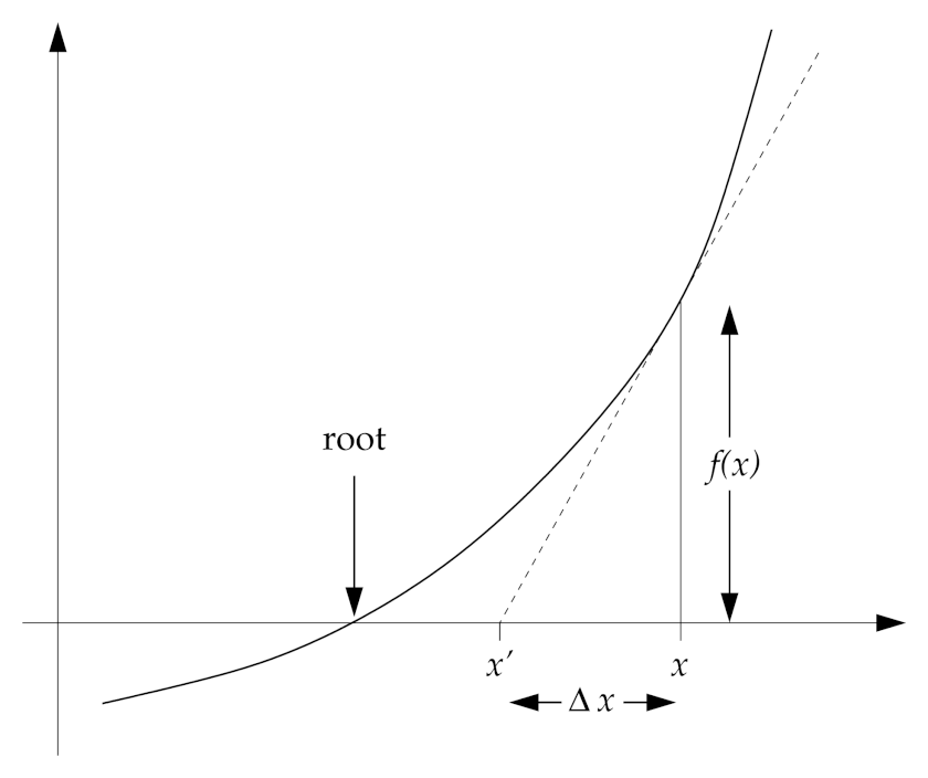
| EPS | PNG | 6.5 | A function with a double root
|
| EPS | PNG | 6.6 | Newton's method
|
| EPS | PNG | 6.7 | Failure of Newton's method
|
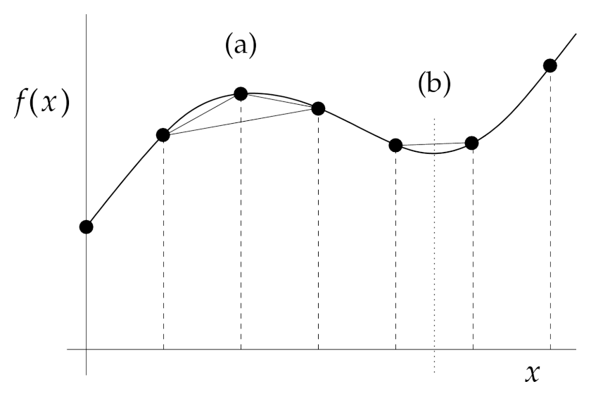
| EPS | PNG | 6.8 | Local and global minima of a function
|
| EPS | PNG | 6.9 | Golden ratio search
|
Chapter 7: Fourier transforms
| EPS | PNG | 7.1 | Creating a periodic function from a nonperiodic one
|
| EPS | PNG | 7.2a | Sample positions for Type-I DFT
|
| EPS | PNG | 7.2b | Sample positions for Type-II DFT
|
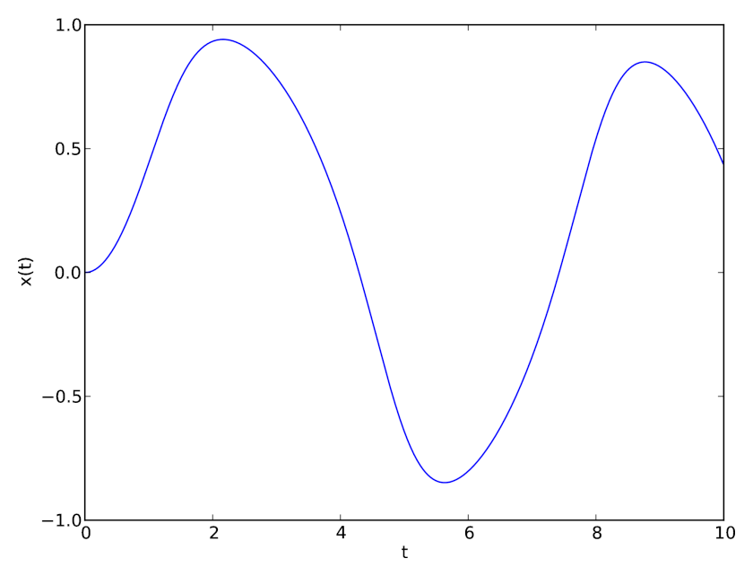
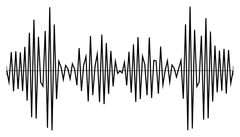
| EPS | PNG | 7.3 | An example signal
|
| EPS | PNG | 7.4 | Fourier transform of Fig. 7.3
|
| EPS | PNG | 7.5 | Turning a nonsymmetric function into a symmetric one
|
Chapter 8: Ordinary differential equations
| EPS | PNG | 8.1 | Numerical solution of an ordinary differential equation
|
| EPS | PNG | 8.2 | Euler's method and the second-order Runge-Kutta method
|
| EPS | PNG | 8.3 | Solutions calculated with the second-order Runge-Kutta method
|
| EPS | PNG | 8.4 | Solutions calculated with the fourth-order Runge-Kutta method
|
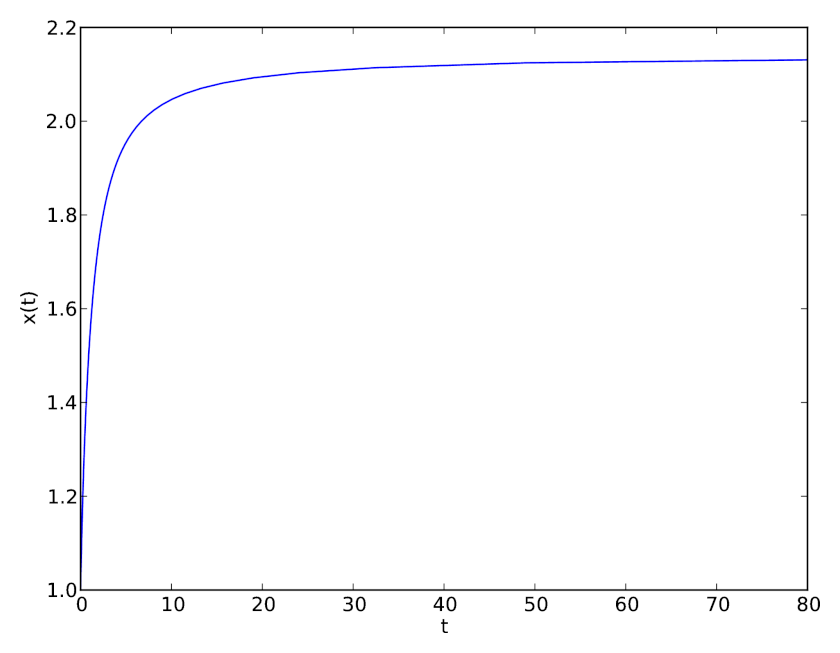
| EPS | PNG | 8.5 | Solution of a differential equation to infinity
|
| EPS | PNG | 8.6 | Adaptive step sizes
|
| EPS | PNG | 8.7 | The adaptive step size method
|
| EPS | PNG | 8.8 | Motion of a nonlinear pendulum
|
| EPS | PNG | 8.9 | Second-order Runge-Kutta and the leapfrog method
|
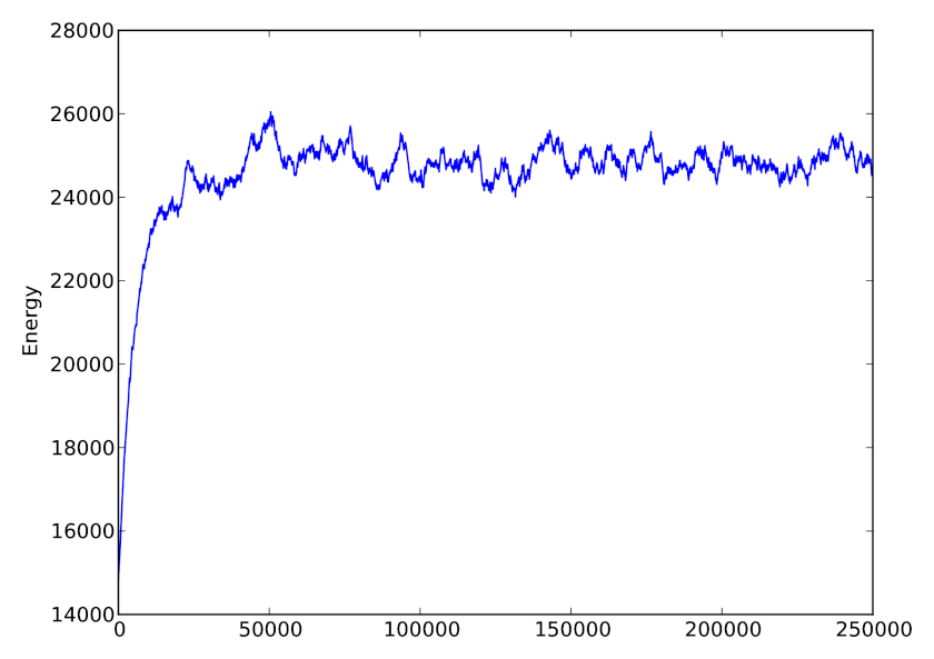
| EPS | PNG | 8.10 | Total energy of the nonlinear pendulum
|
| EPS | PNG | 8.11 | The shooting method
|
| EPS | PNG | 8.12 | Solution of the Schrodinger equation in a square well
|
Chapter 9: Partial differential equations
| EPS | PNG | 9.1 | A simple electrostatics problem
|
| EPS | PNG | 9.2 | Finite differences
|
| EPS | PNG | 9.3 | Solution of the Laplace equation
|
| EPS | PNG | 9.4 | A more complicated electrostatics problem
|
| EPS | PNG | 9.5 | Solution for the electrostatic potential of Fig. 9.4
|
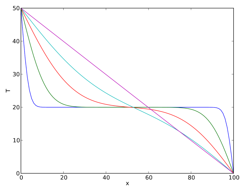
| EPS | PNG | 9.6 | Solution of the heat equation
|
| EPS | PNG | 9.7a | FTCS solution of the wave equation (a)
|
| EPS | PNG | 9.7b | FTCS solution of the wave equation (b)
|
| EPS | PNG | 9.7c | FTCS solution of the wave equation (c)
|
Chapter 10: Random processes and Monte Carlo methods
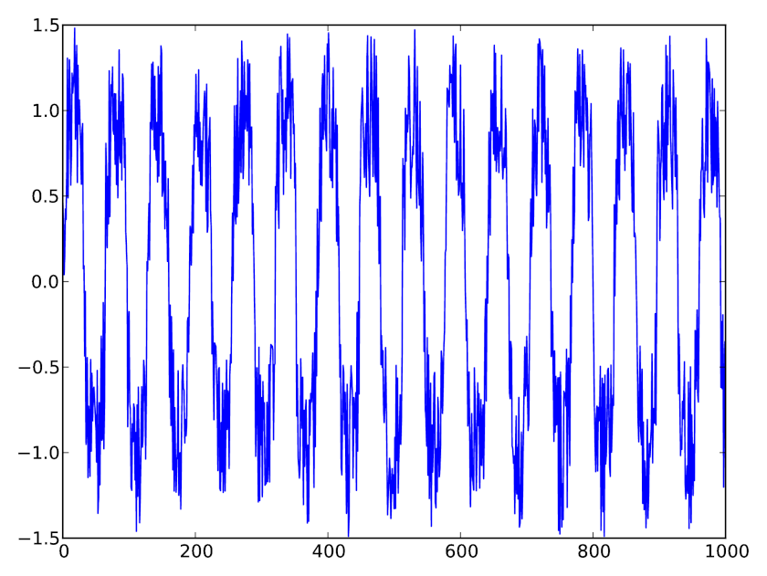
| EPS | PNG | 10.1 | Output of the linear congruential random number generator
|
| EPS | PNG | 10.2 | Decay of a sample of radioactive atoms
|
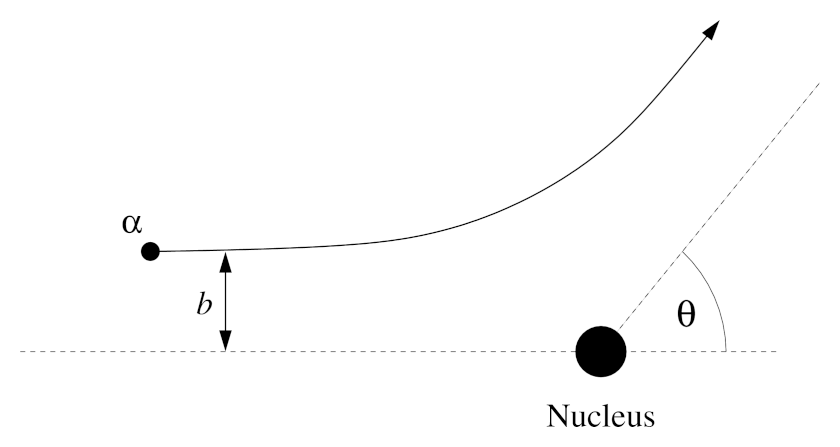
| EPS | PNG | 10.3 | Rutherford scattering
|
| EPS | PNG | 10.4 | A pathological function
|
| EPS | PNG | 10.5 | Internal energy of an ideal gas
|
| EPS | PNG | 10.6 | The traveling salesman problem
|
| EPS | PNG | 10.7a | Solution of a random traveling salesman problem
|
| EPS | PNG | 10.7b | Solution of another random traveling salesman problem
|