Figures
This page contains figures from the book Computational Physics, 2nd edition, by Mark Newman. You can also download all figures in a single ZIP file here. A few figures are not included because of licensing limitations.
Chapter 2: Python programming for physicists
| Format | Figure | Description |
|---|
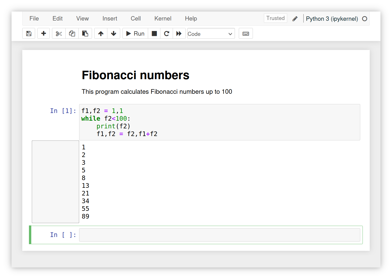
| – | PNG | 2.1 | Jupyter notebook
|
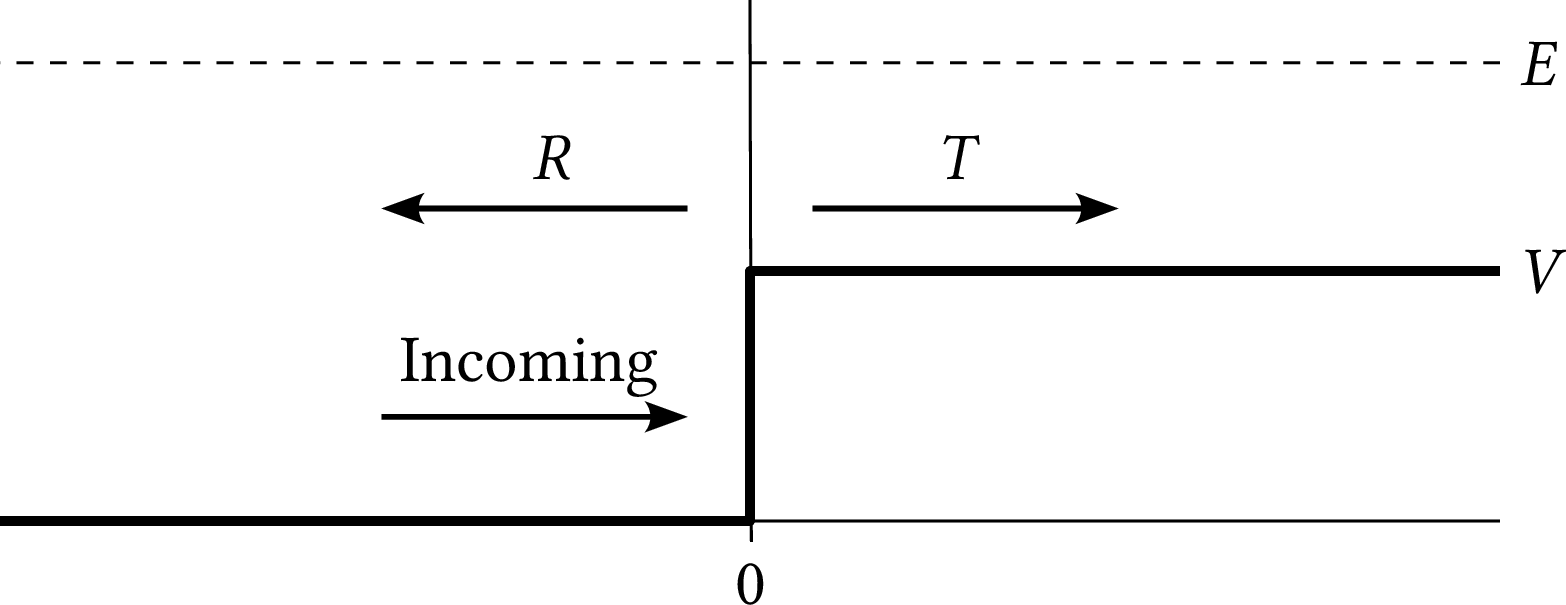
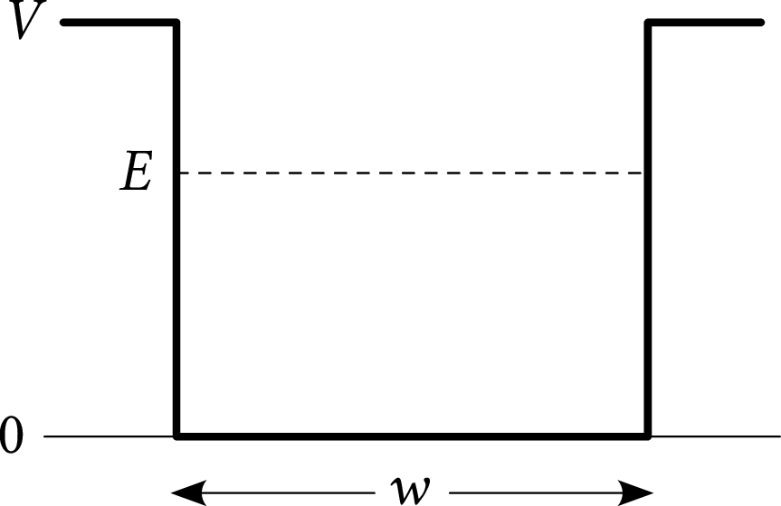
| PDF | PNG | – | Potential step
|
Chapter 3: Graphics and visualization
| Format | Figure | Description |
|---|
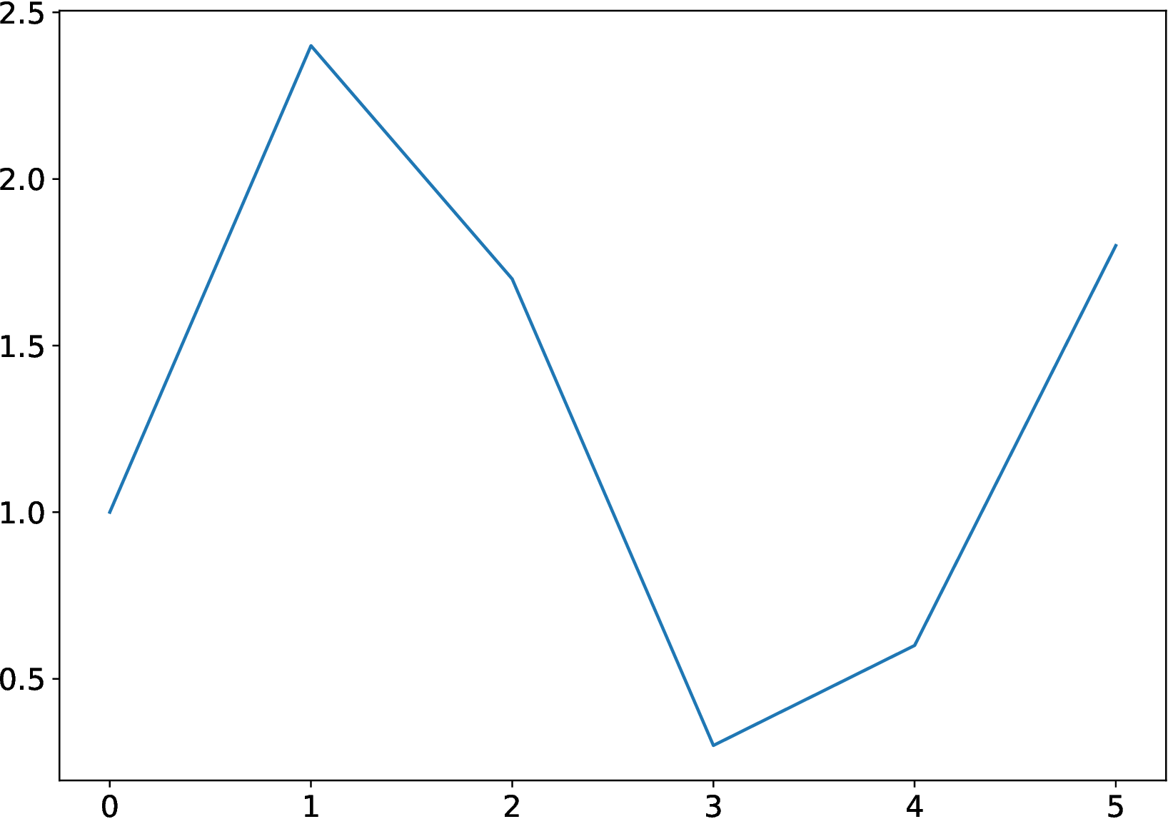
| PDF | PNG | – | Example graph 1
|
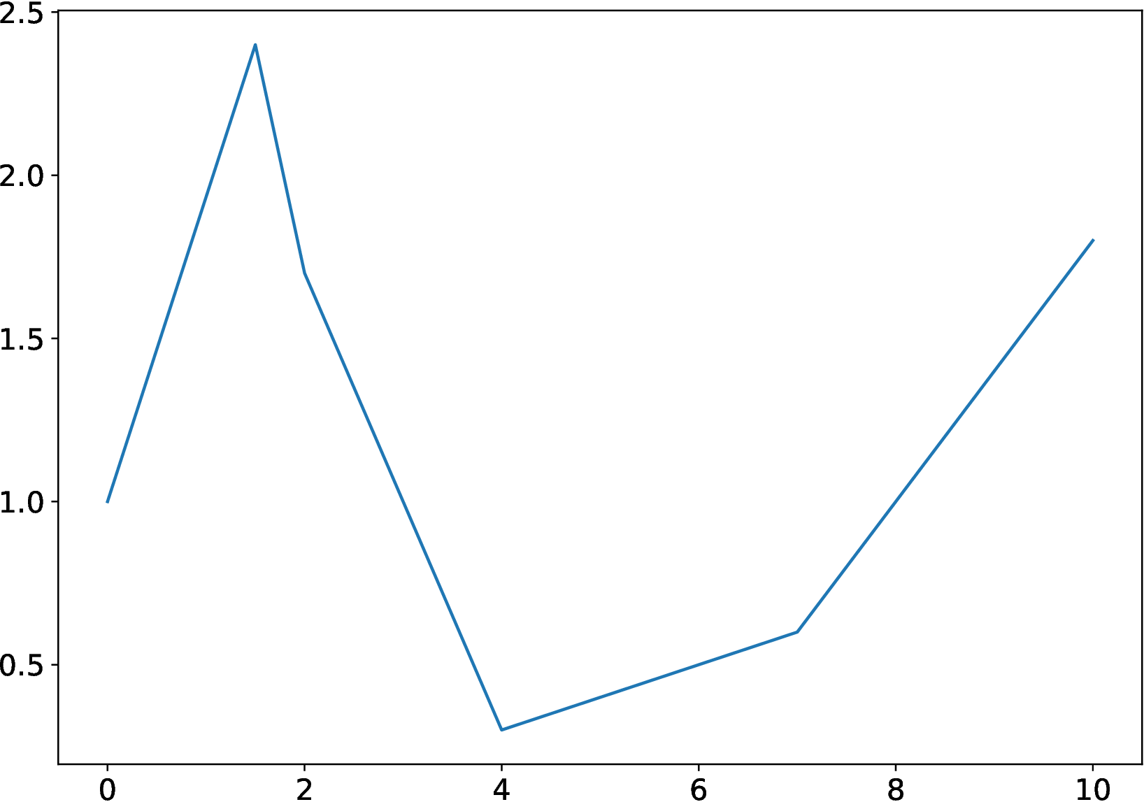
| PDF | PNG | – | Example graph 2
|
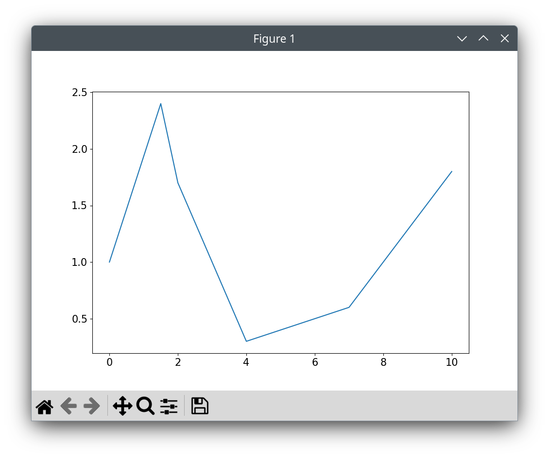
| – | PNG | 3.1 | Matplotlib graph window
|
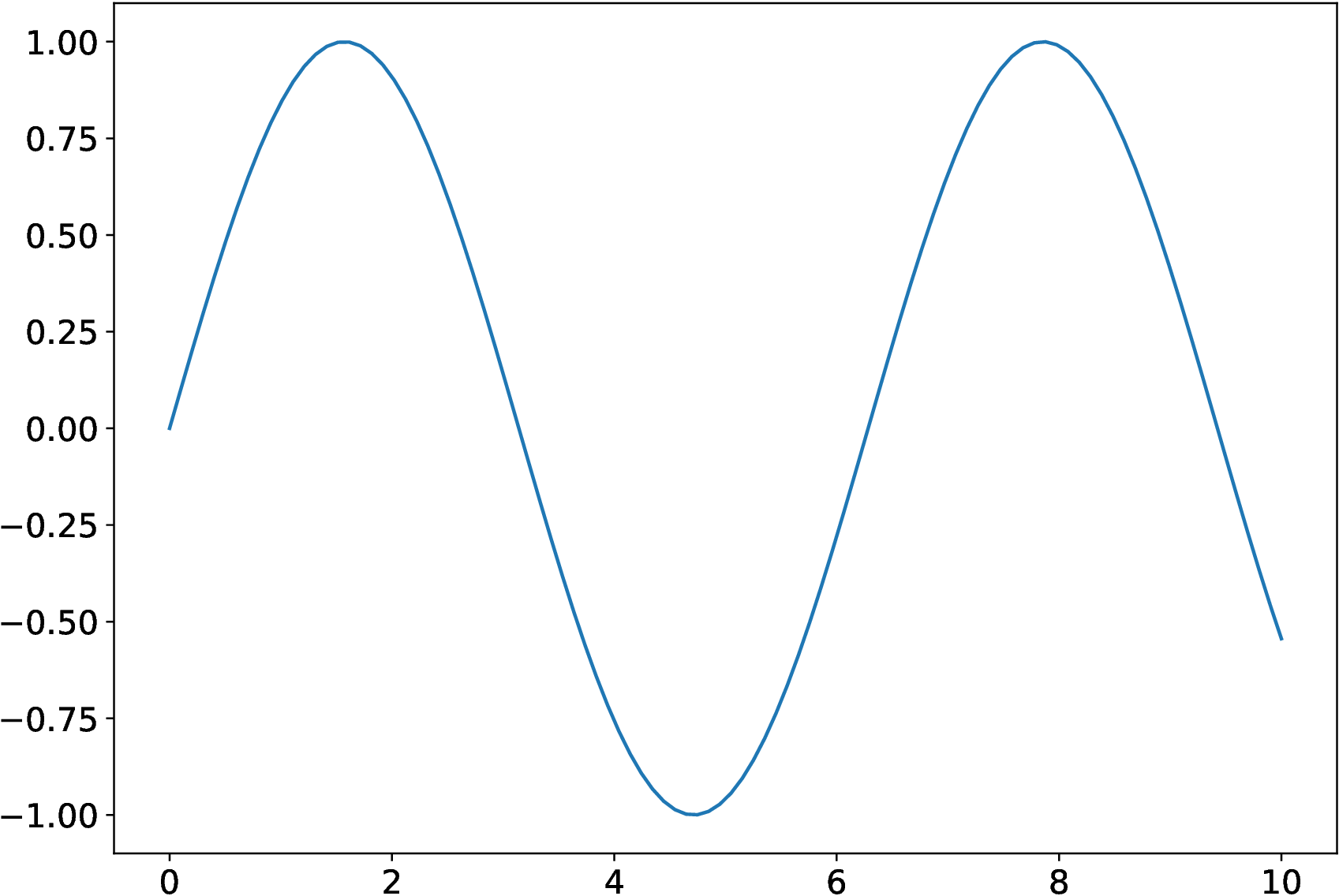
| PDF | PNG | 3.2 | Graph of sine function
|
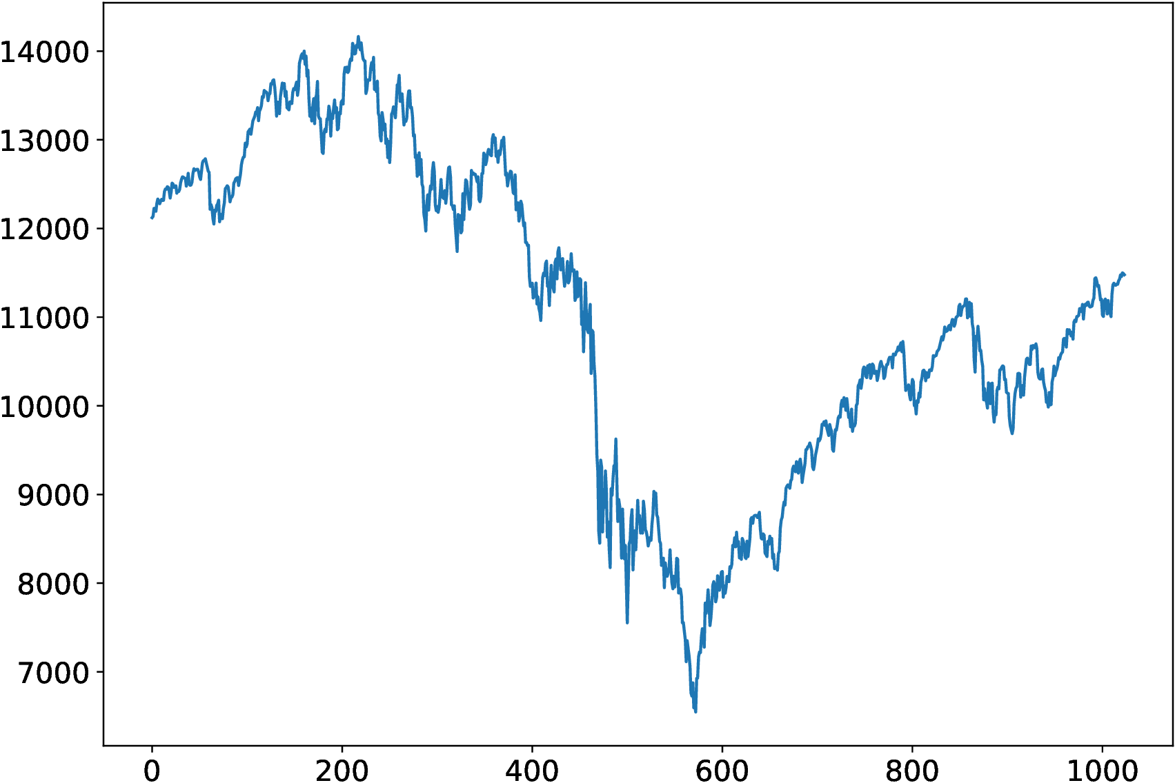
| PDF | PNG | 3.3 | Graph of data from a file
|
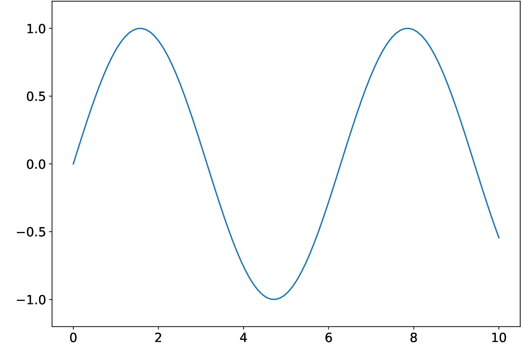
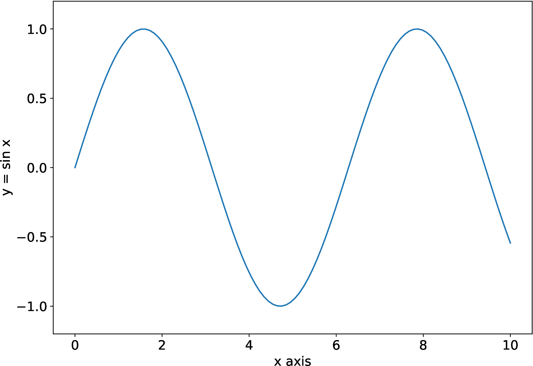
| PDF | PNG | 3.4a | Sine function, version 1
|
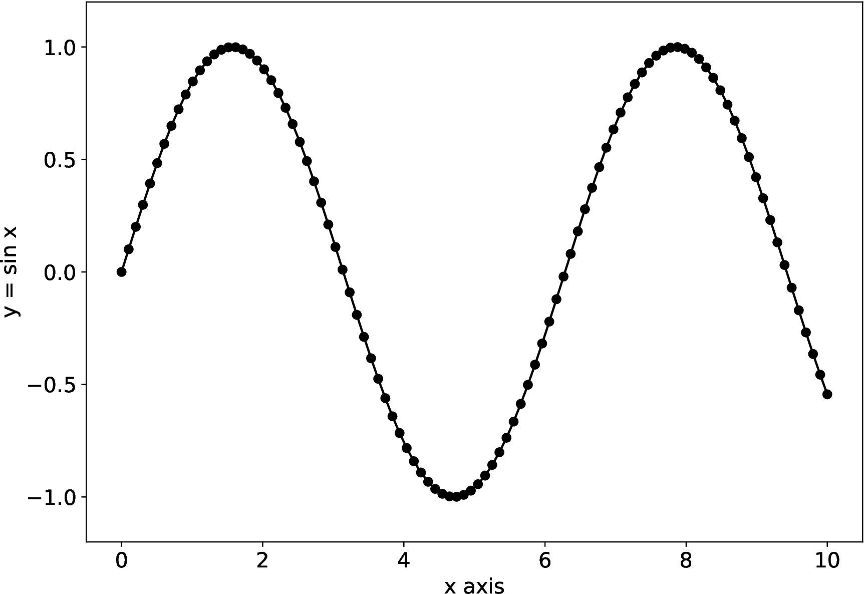
| PDF | PNG | 3.4b | Sine function, version 2
|
| PDF | PNG | 3.4c | Sine function, version 3
|
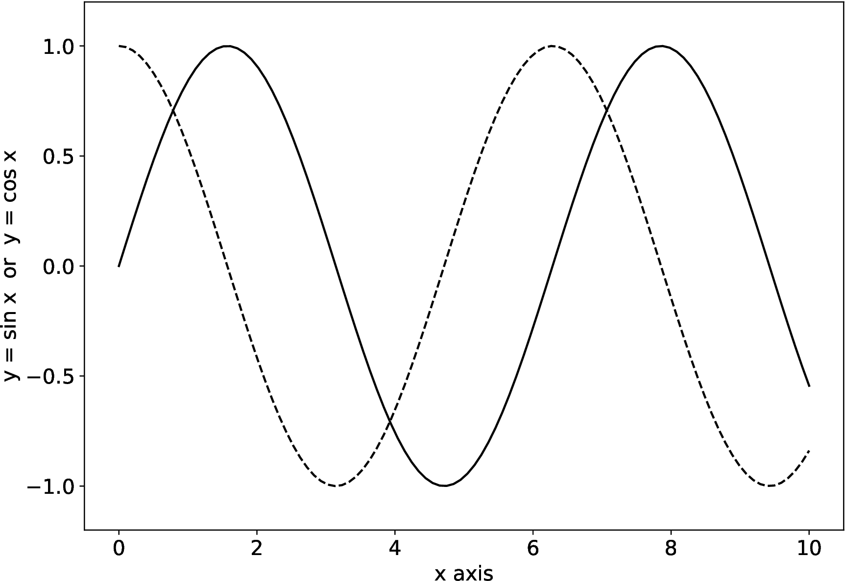
| PDF | PNG | 3.4d | Sine and cosine functions
|
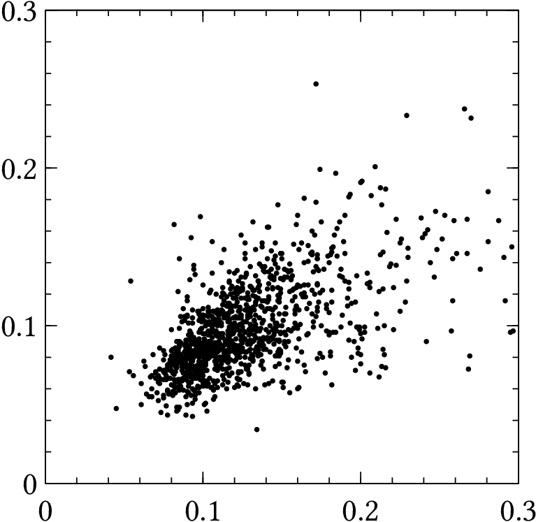
| PDF | PNG | – | Scatter plot
|
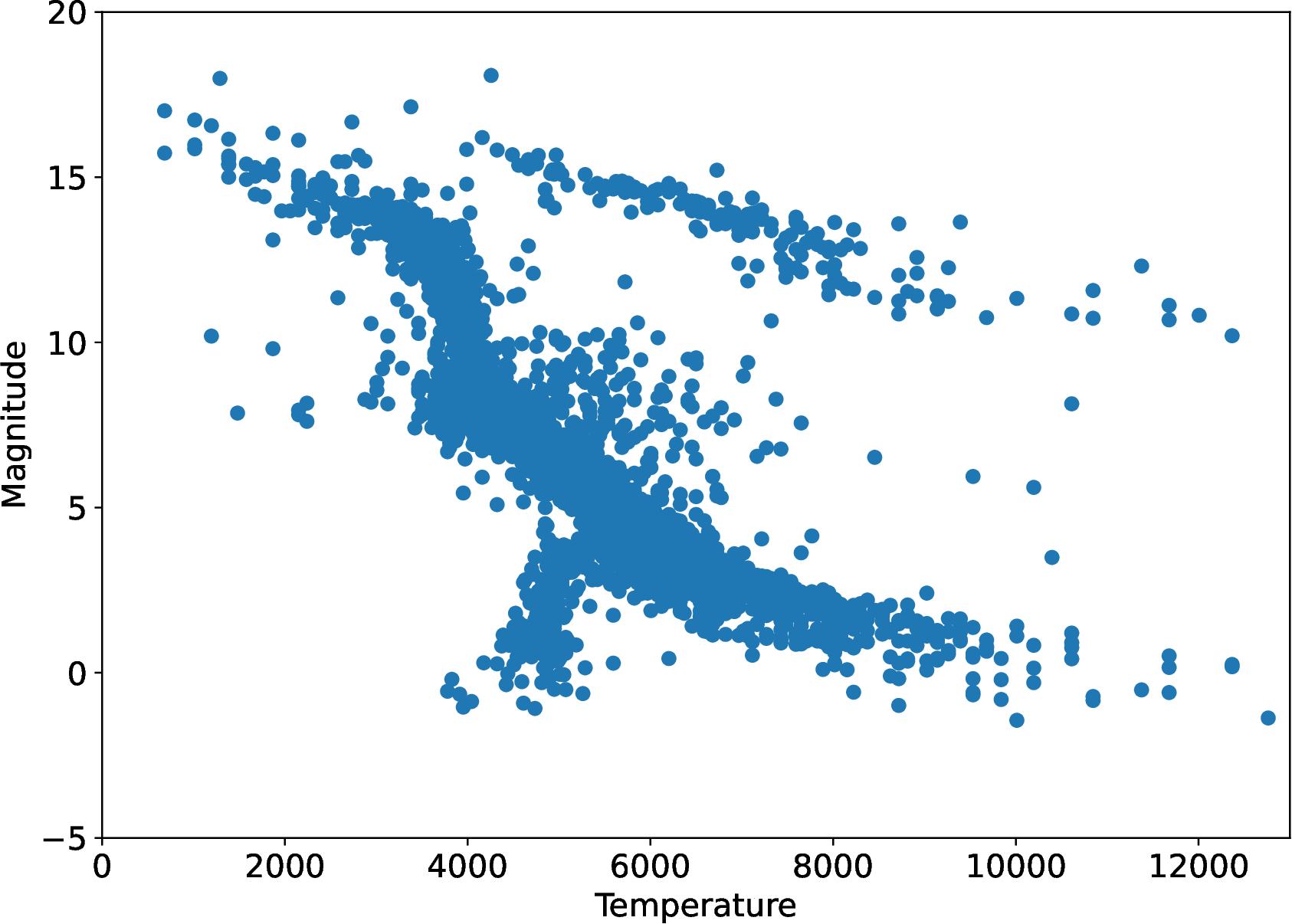
| PDF | PNG | 3.5 | Hertzsprung-Russell diagram
|
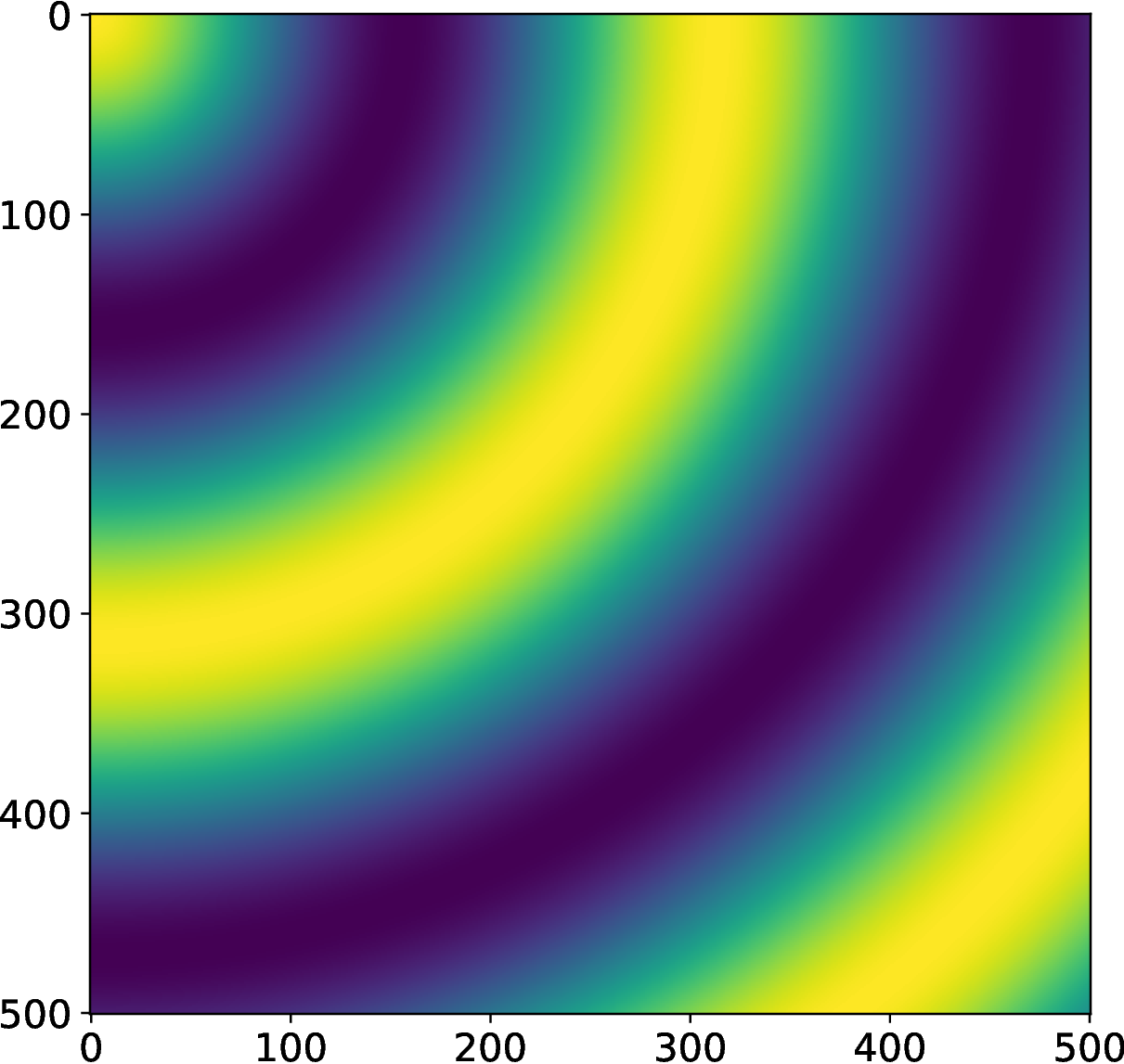
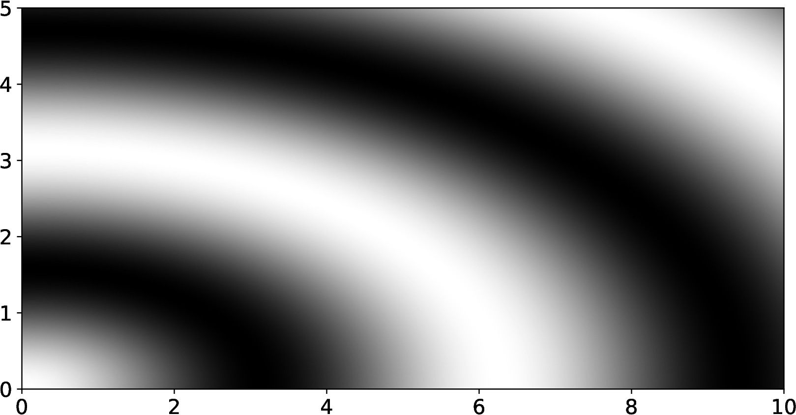
| PDF | PNG | 3.6 | Density plot example
|
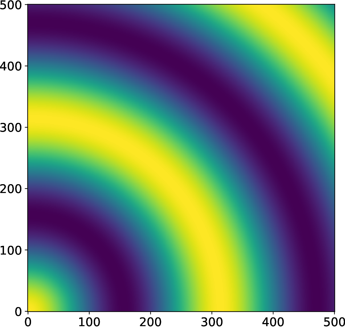
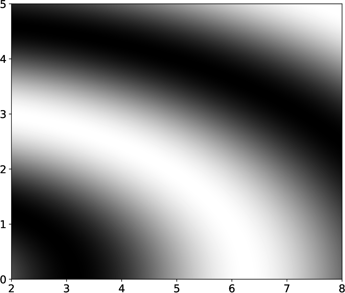
| PDF | PNG | 3.7a | Density plot, version 1
|
| PDF | PNG | 3.7b | Density plot, version 2
|
| PDF | PNG | 3.7c | Density plot, version 3
|
| PDF | PNG | 3.7d | Density plot, version 4
|
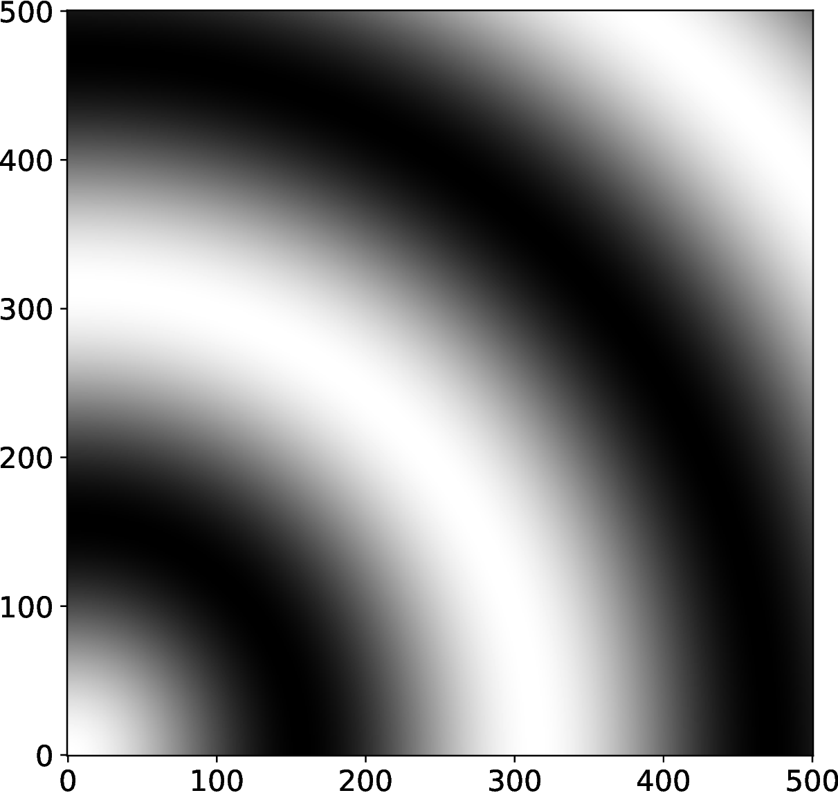
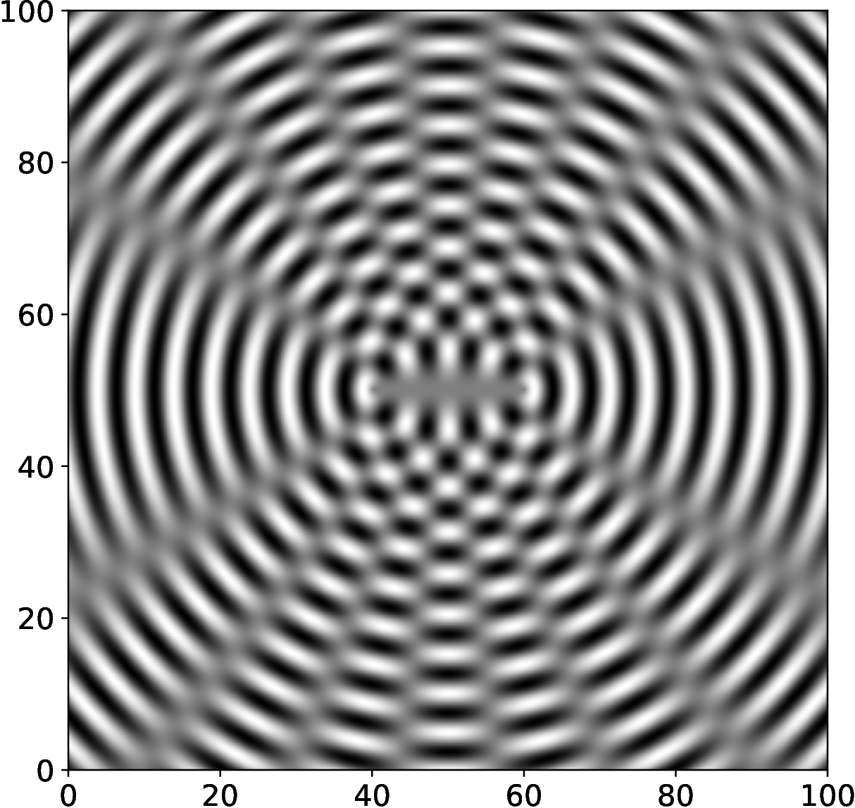
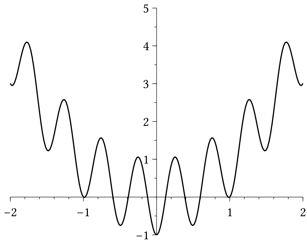
| PDF | PNG | 3.8 | Wave interference
|
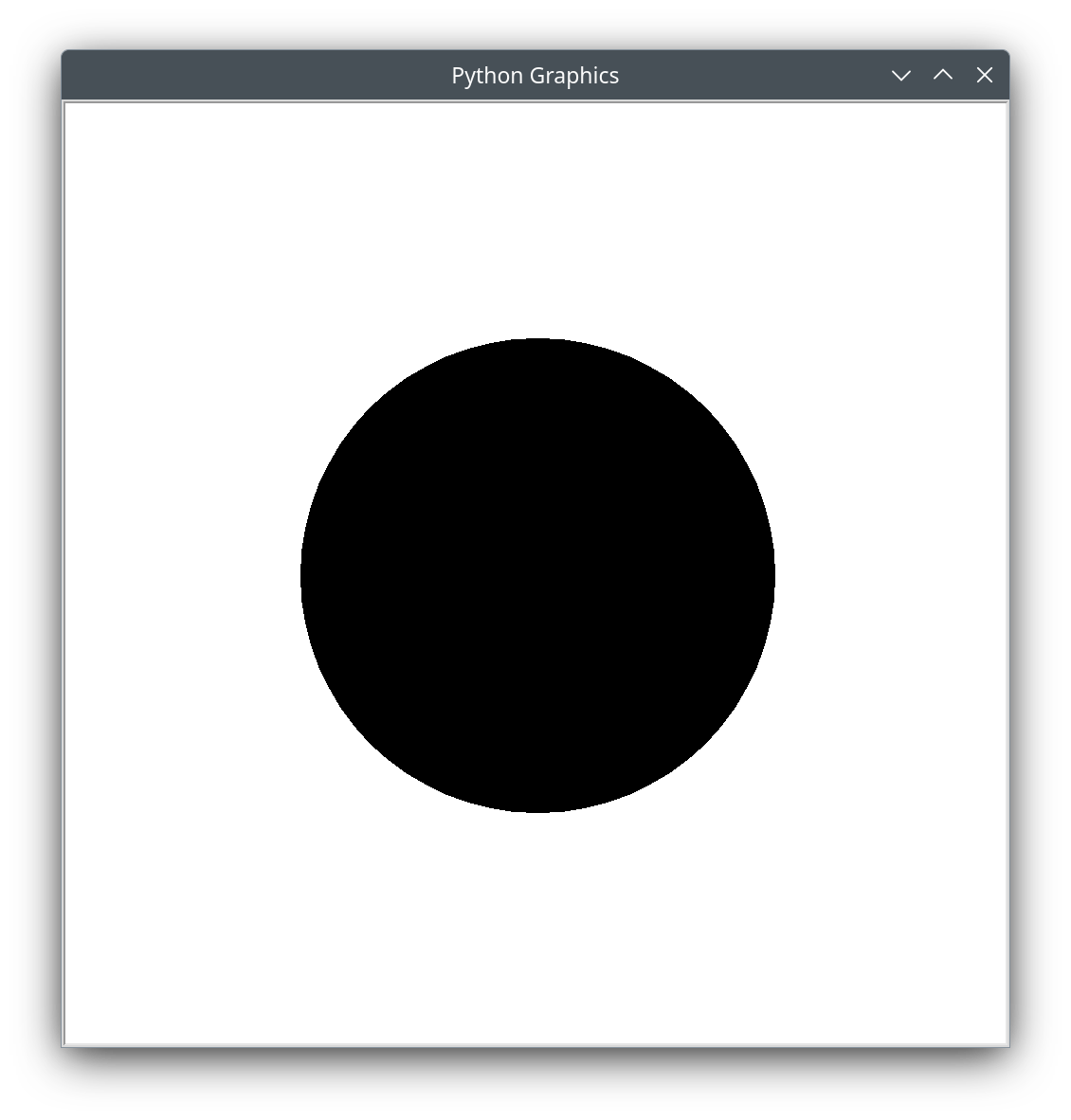
| – | PNG | 3.9 | Qdraw graphics window
|
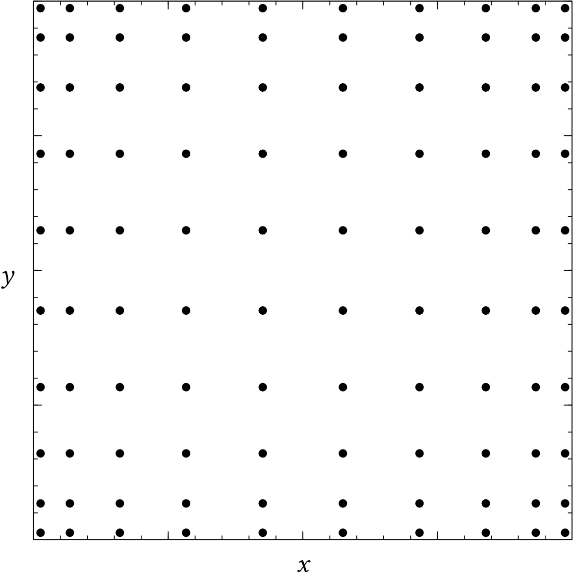
| – | PNG | 3.10 | Atoms in a square lattice
|
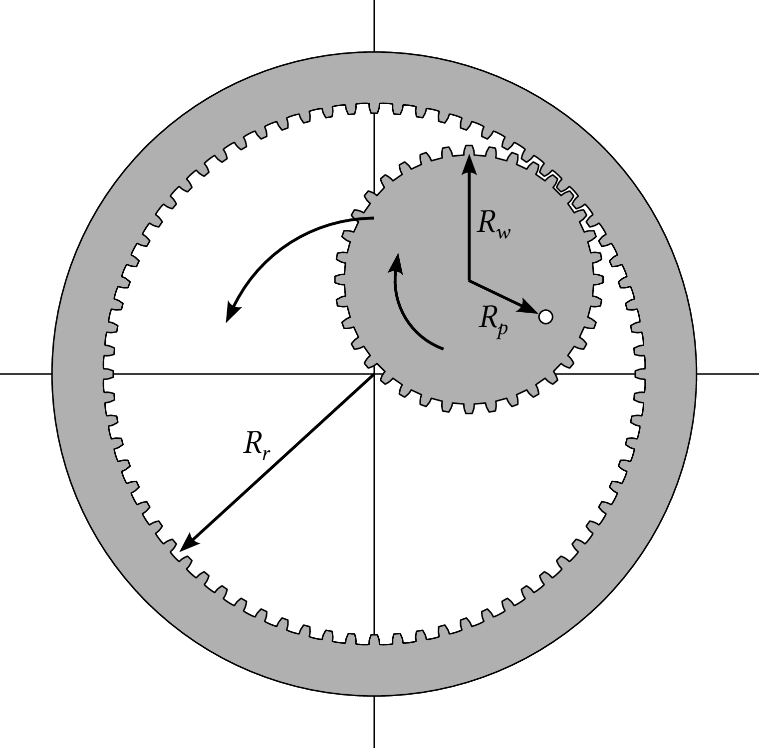
| PDF | PNG | 3.11 | Spirograph
|
Chapter 4: Accuracy and speed
| Format | Figure | Description |
|---|
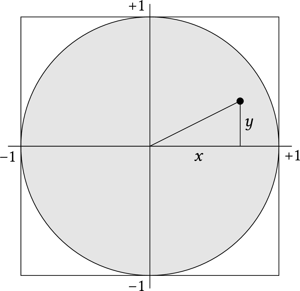
| PDF | PNG | 4.1 | Area under a semicircle
|
Chapter 5: Integrals and derivatives
| Format | Figure | Description |
|---|
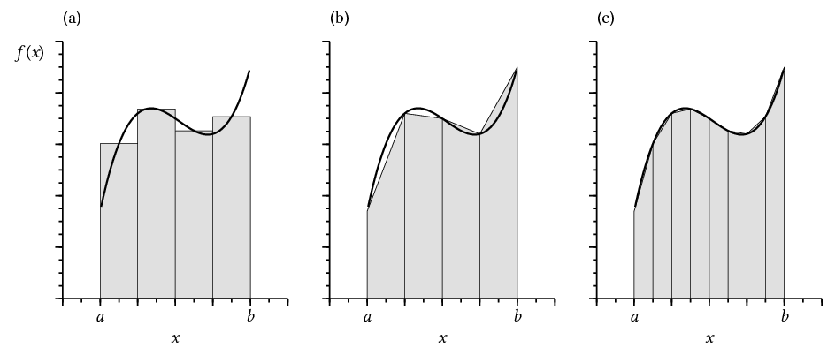
| PDF | PNG | 5.1 | Estimating the area under a curve
|
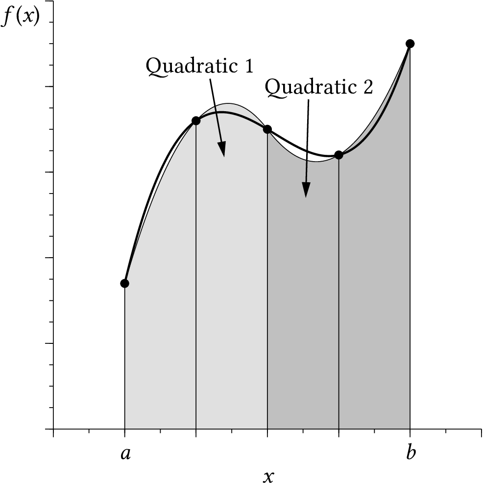
| PDF | PNG | 5.2 | Simpson's rule
|
| PDF | PNG | – | Diffraction pattern
|
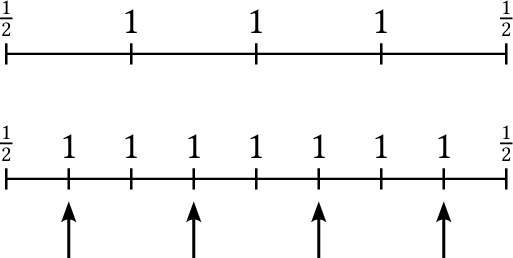
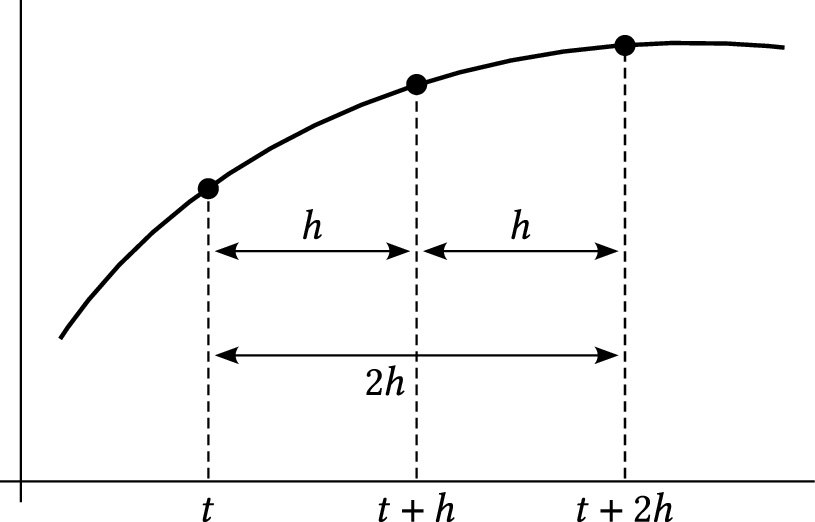
| PDF | PNG | 5.3 | Doubling the number of steps
|
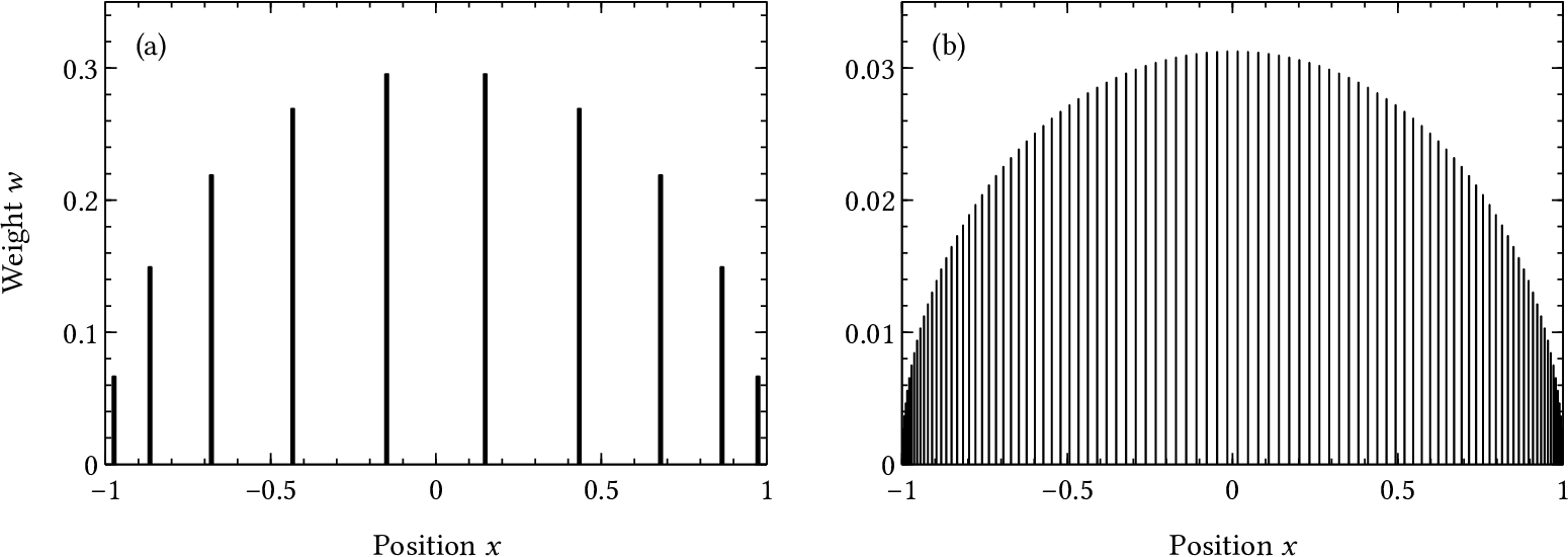
| PDF | PNG | 5.4 | Sample points for Gaussian quadrature
|
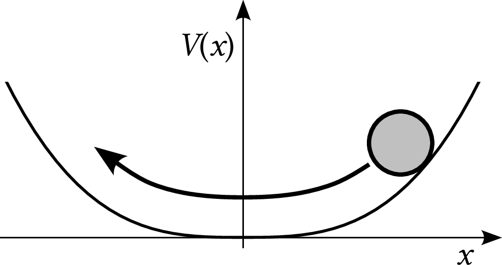
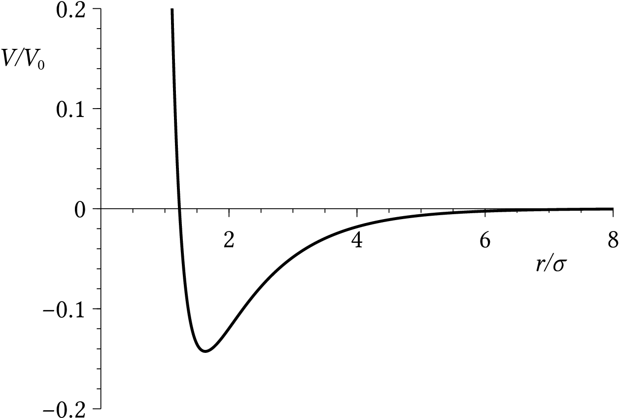
| PDF | PNG | – | Anharmonic potential well
|
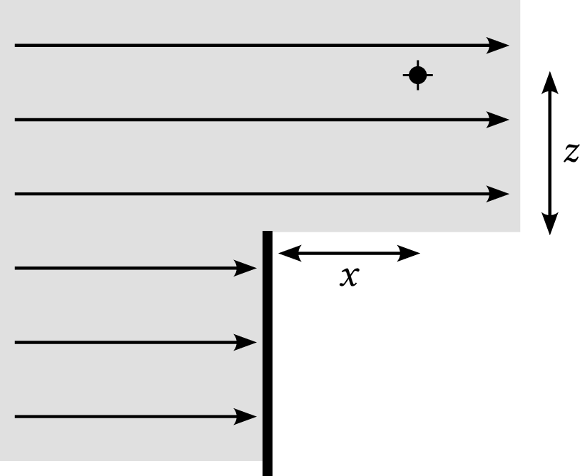
| PDF | PNG | – | Diffraction at a straight edge
|
| PDF | PNG | 5.5 | Gaussian quadrature in 2D
|
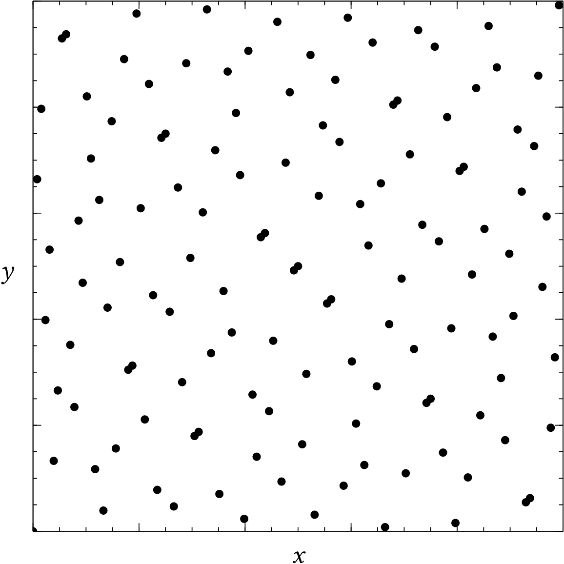
| PDF | PNG | 5.6 | Sobol sequence
|
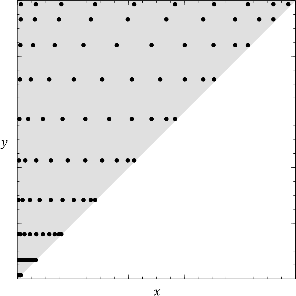
| PDF | PNG | 5.7 | Non-rectangular integration domain
|
| PDF | PNG | 5.8 | Complicated integration domain
|
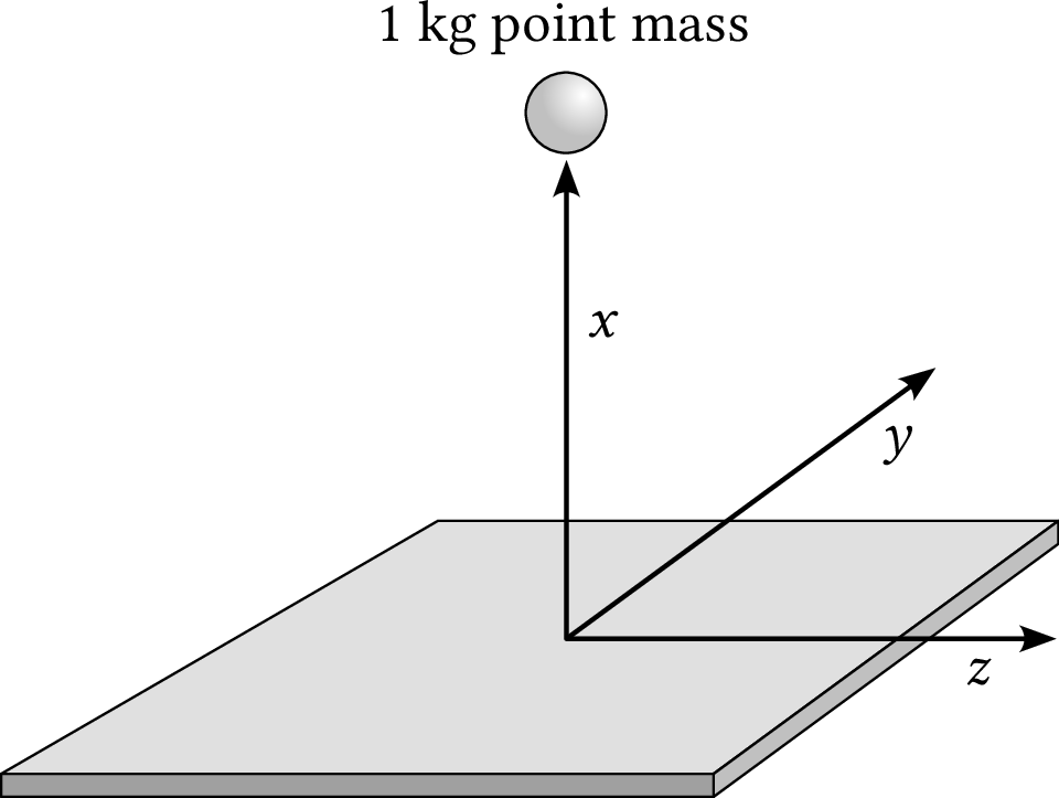
| PDF | PNG | – | Uniform sheet
|
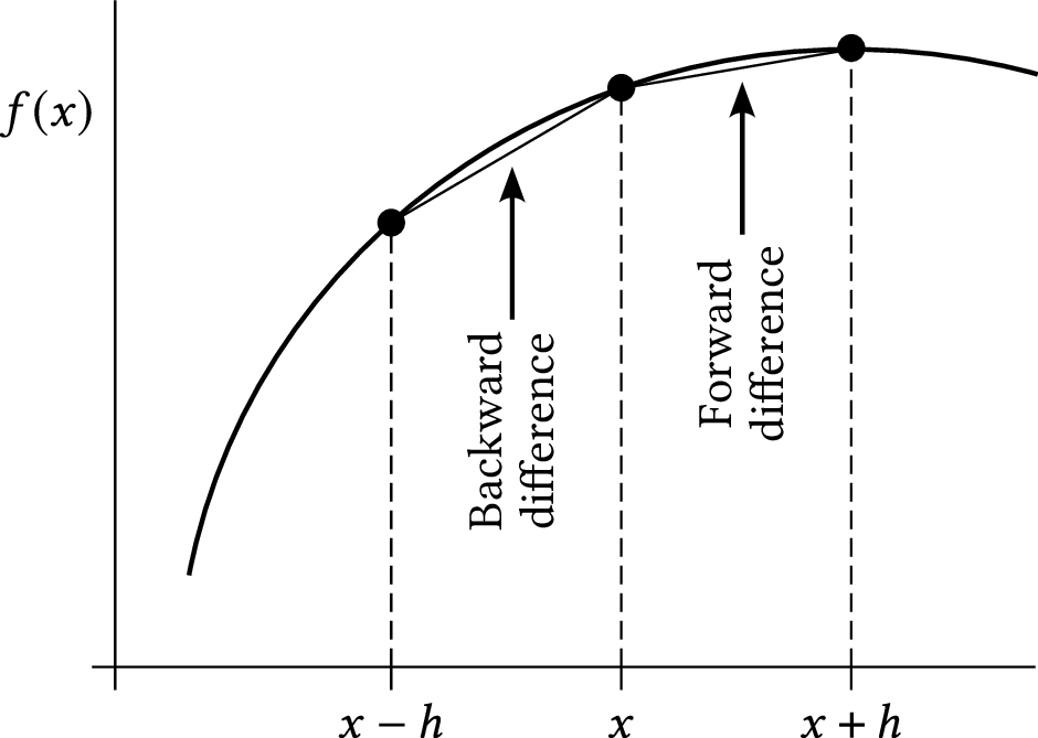
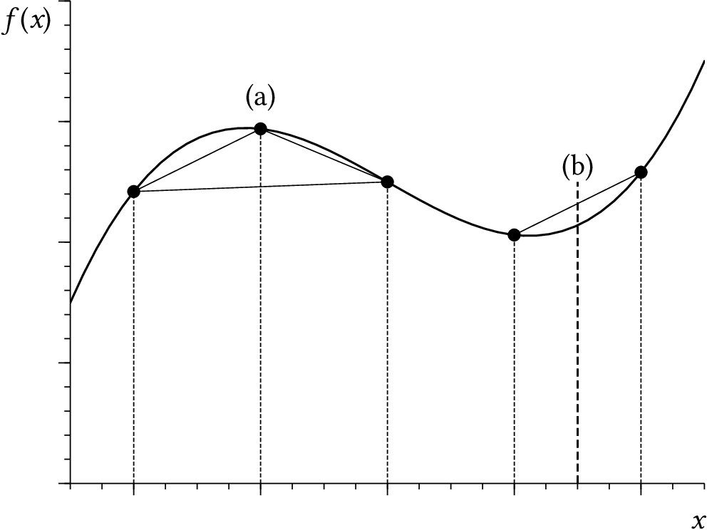
| PDF | PNG | 5.9 | Forward and backward differences
|
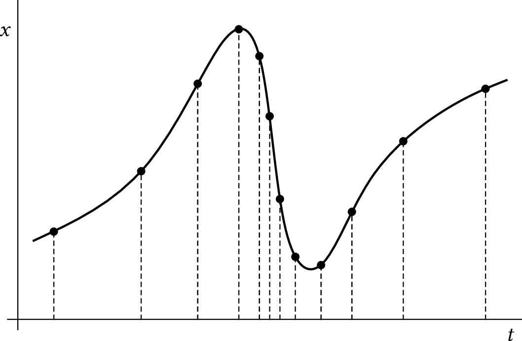
| PDF | PNG | 5.10 | Derivative of a sampled function
|
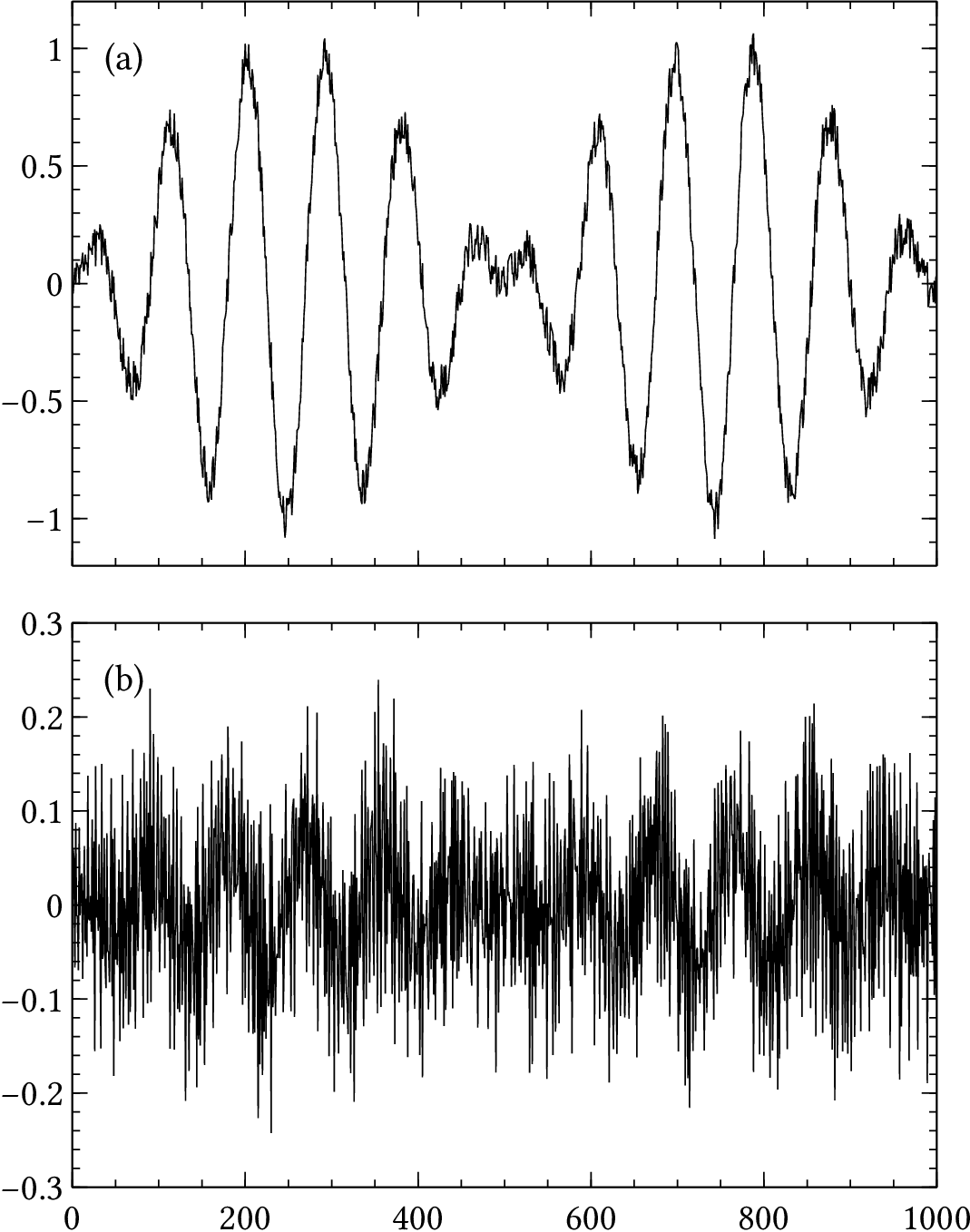
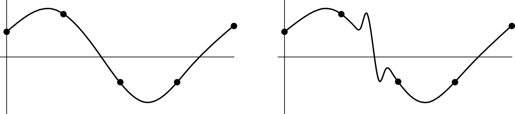
| PDF | PNG | 5.11 | Derivative of noisy data
|
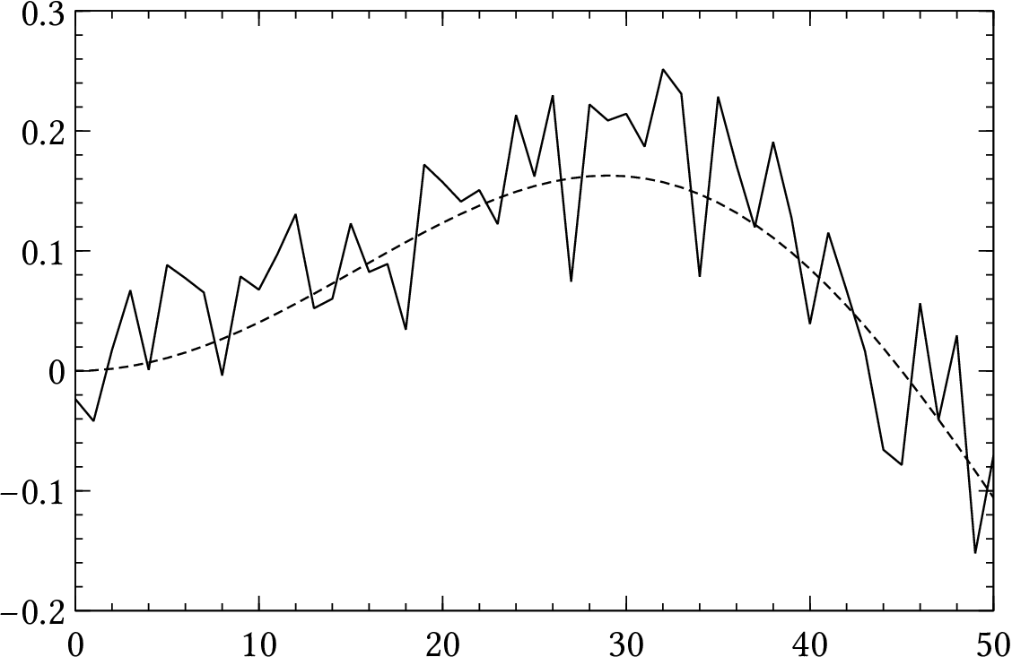
| PDF | PNG | 5.12 | Expanded view of noisy data
|
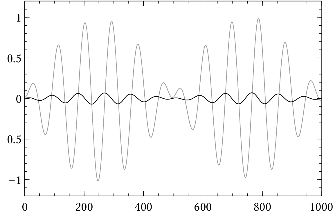
| PDF | PNG | 5.13 | Smoothed version of noisy data
|
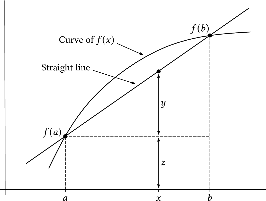
| PDF | PNG | 5.14 | Linear interpolation
|
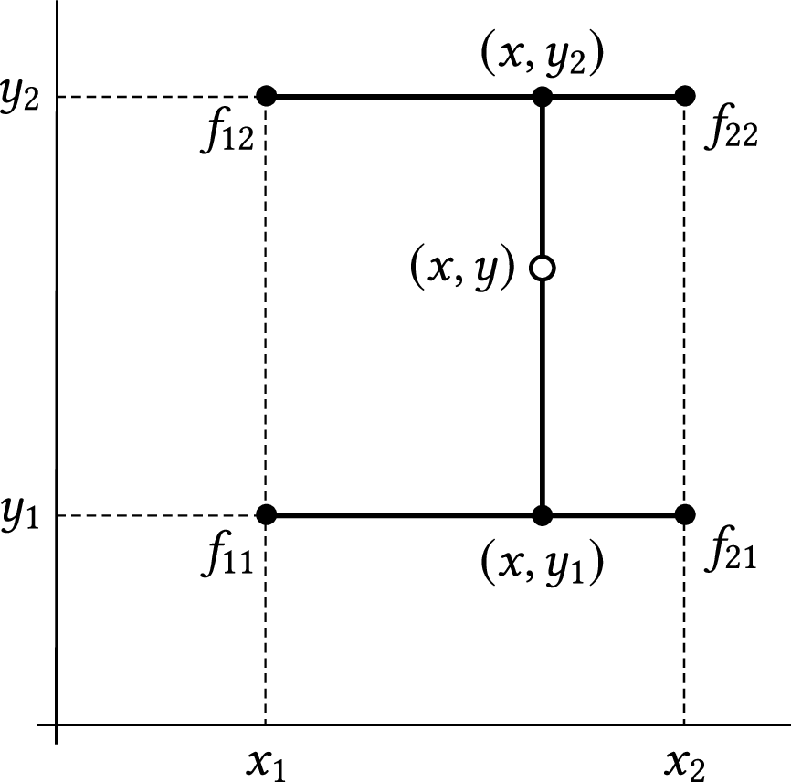
| PDF | PNG | 5.15 | Bilinear interpolation
|
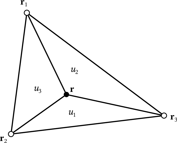
| PDF | PNG | 5.16 | Interpolation in a triangle
|
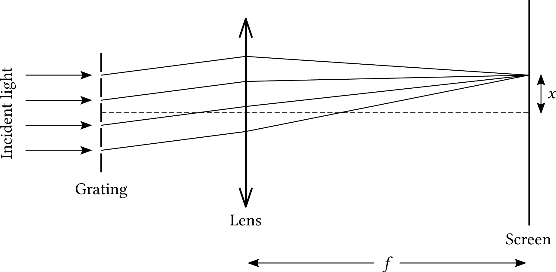
| PDF | PNG | – | Diffraction grating
|
| PDF | PNG | – | Diffraction pattern
|
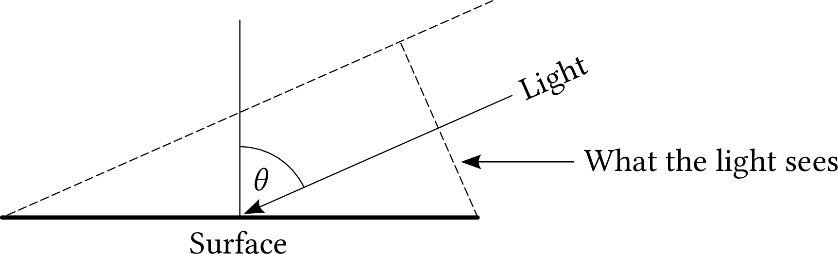
| PDF | PNG | – | Light falling on a surface
|
Chapter 6: Solution of linear and nonlinear equations
Chapter 7: Fourier transforms
| Format | Figure | Description |
|---|
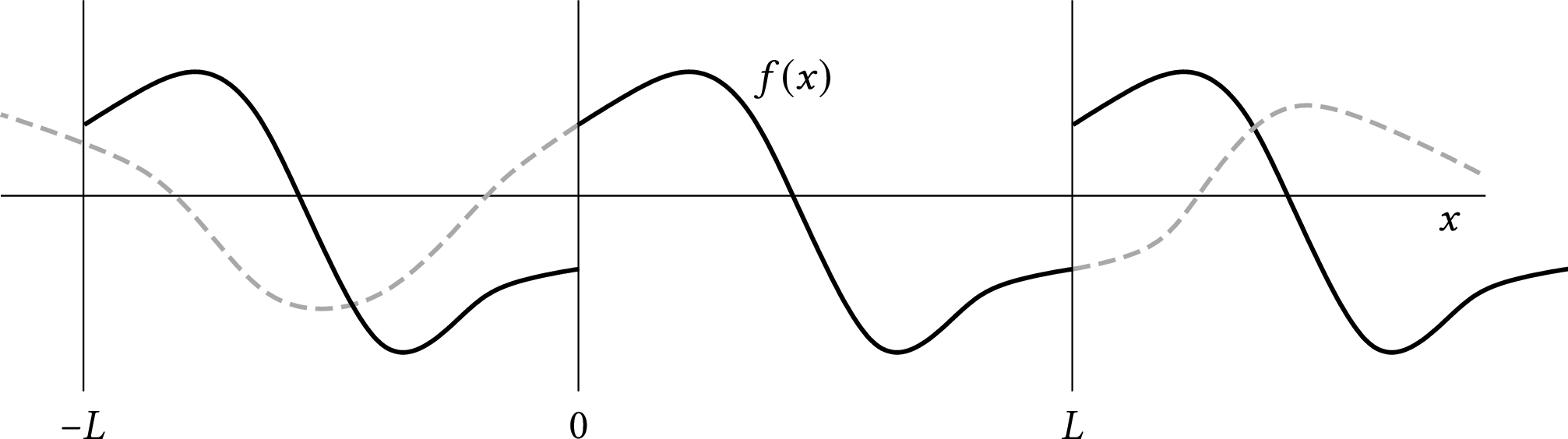
| PDF | PNG | 7.1 | Creating a periodic function
|
| PDF | PNG | – | Functions with the same samples
|
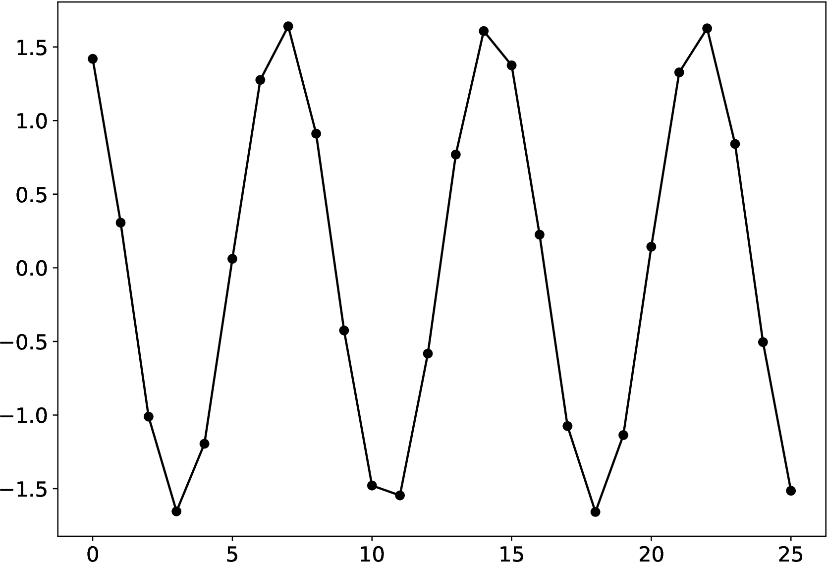
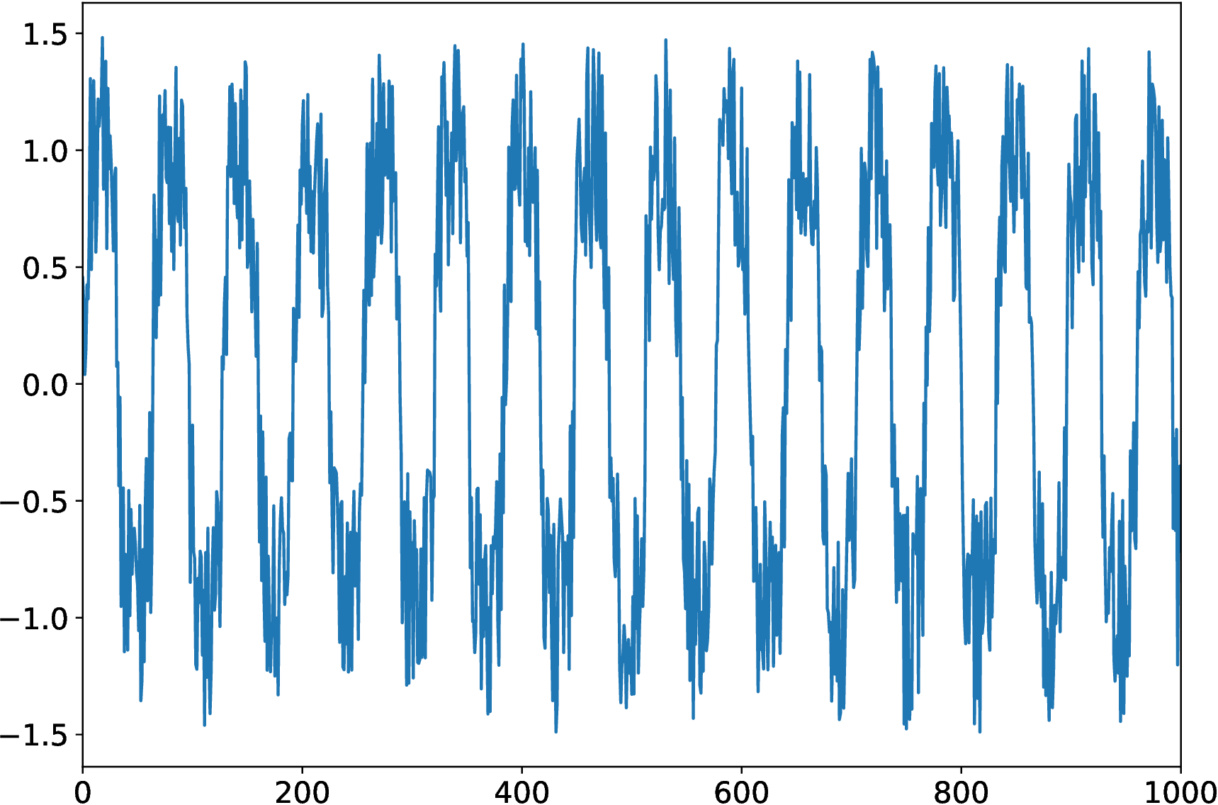
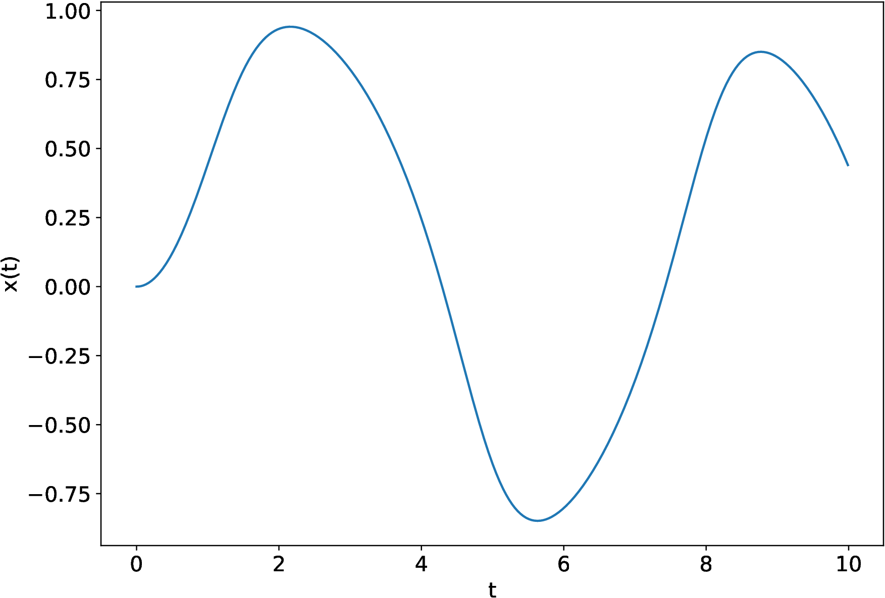
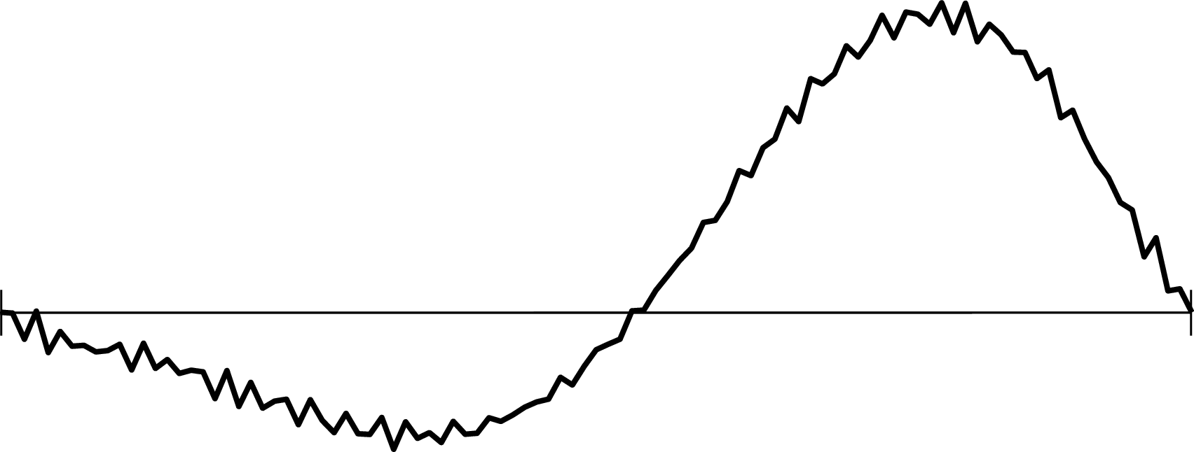
| PDF | PNG | 7.2 | Example signal
|
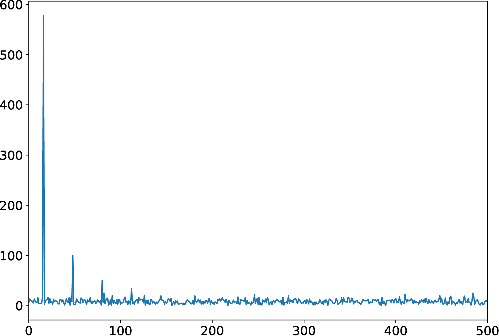
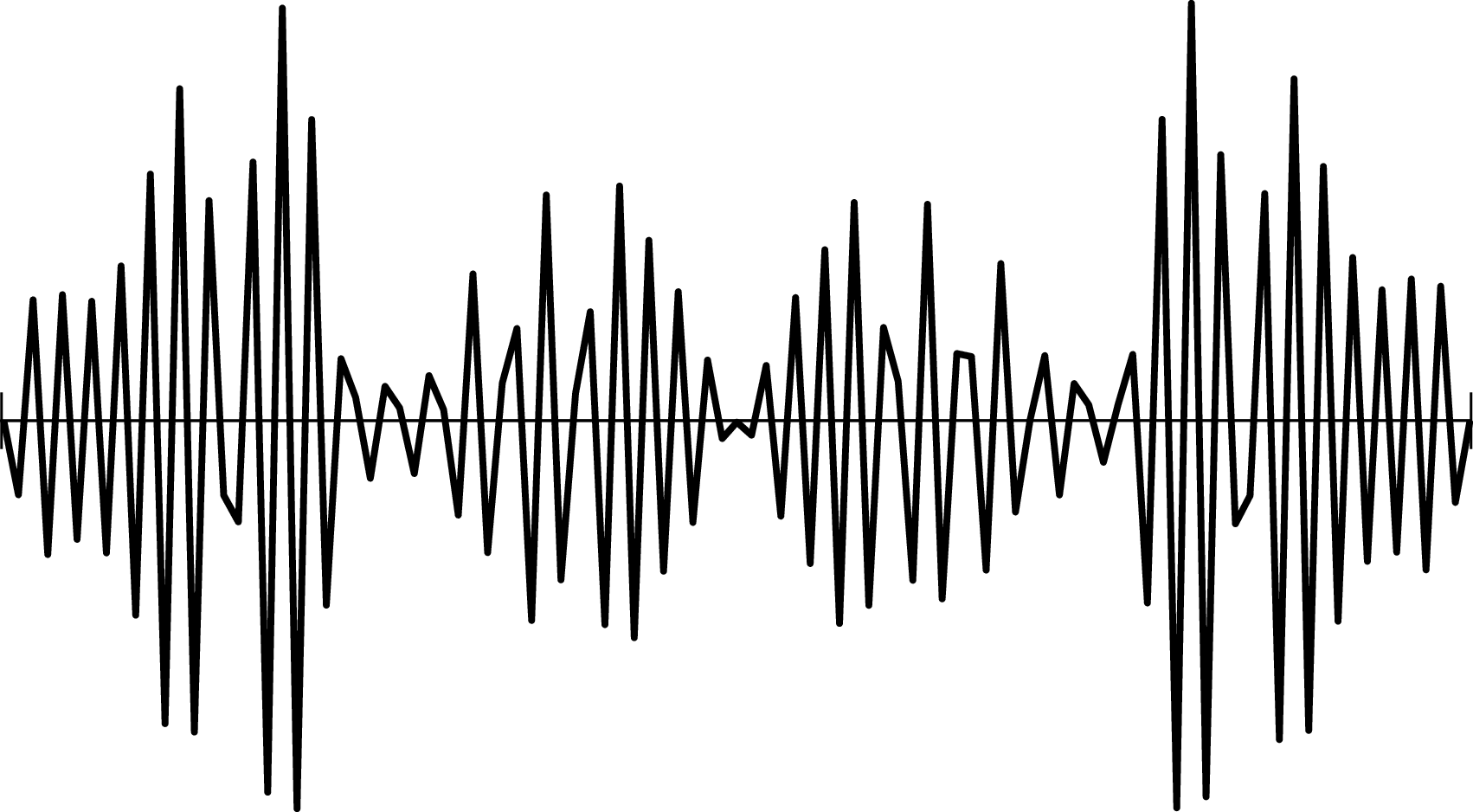
| PDF | PNG | 7.3 | Fourier transform of Fig. 7.2
|
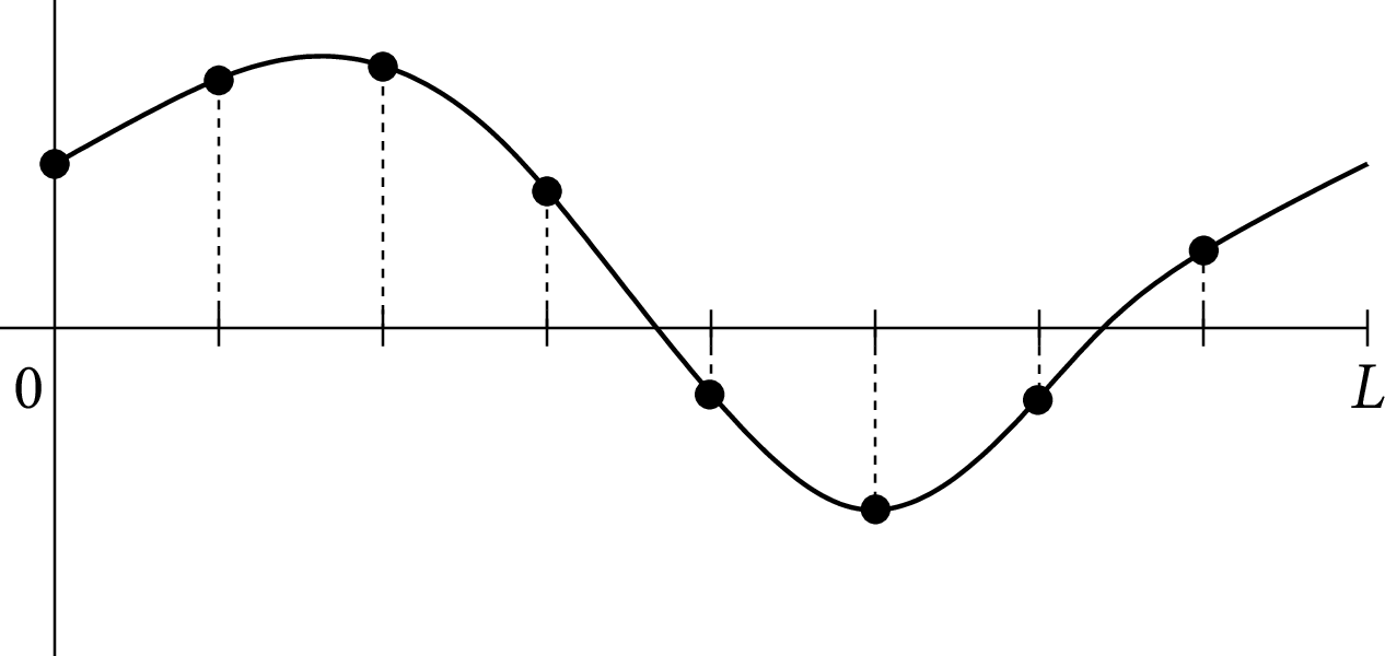
| PDF | PNG | 7.4a | Type-I DFT
|
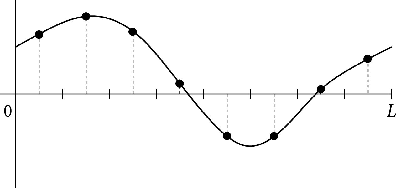
| PDF | PNG | 7.4b | Type-II DFT
|
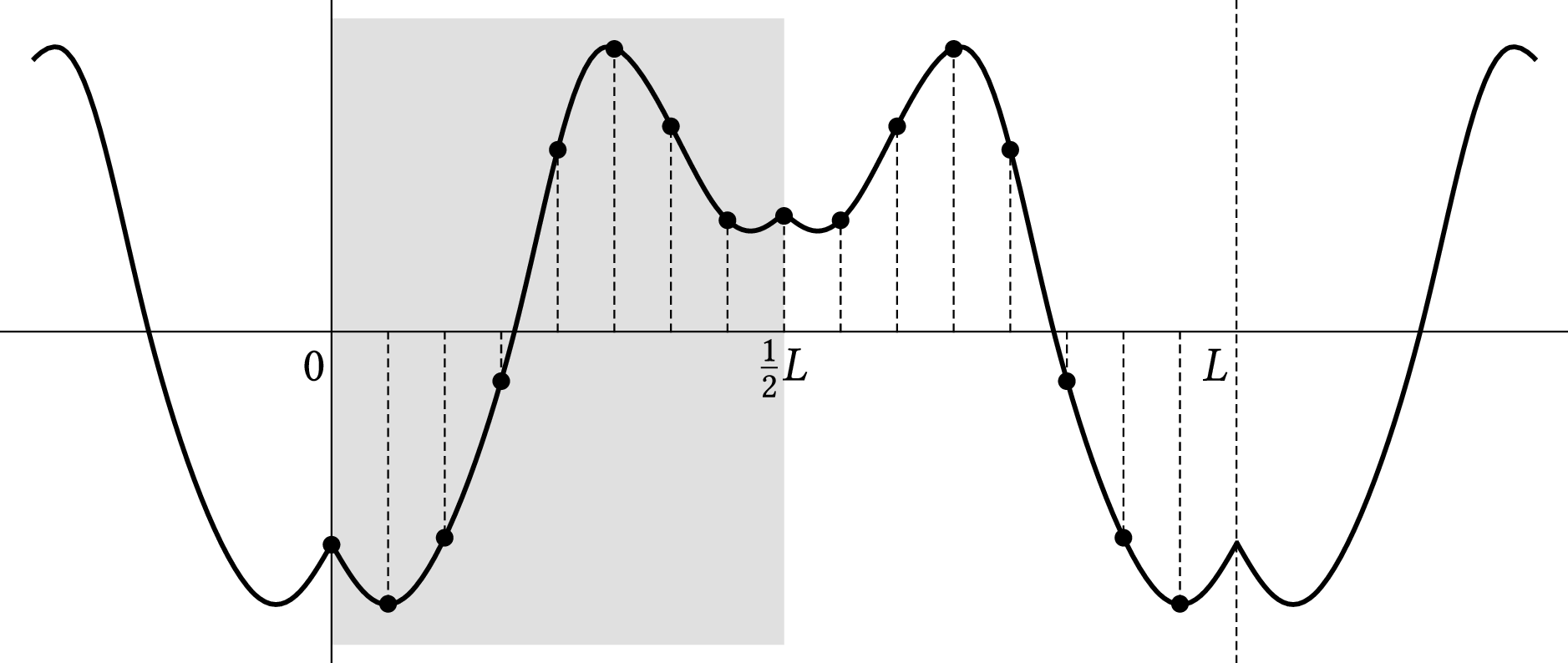
| PDF | PNG | 7.5 | Creating a symmetric function
|
| PDF | PNG | – | Point spread function
|
Chapter 8: Ordinary differential equations
| Format | Figure | Description |
|---|
| PDF | PNG | 8.1 | Solution using Euler's method
|
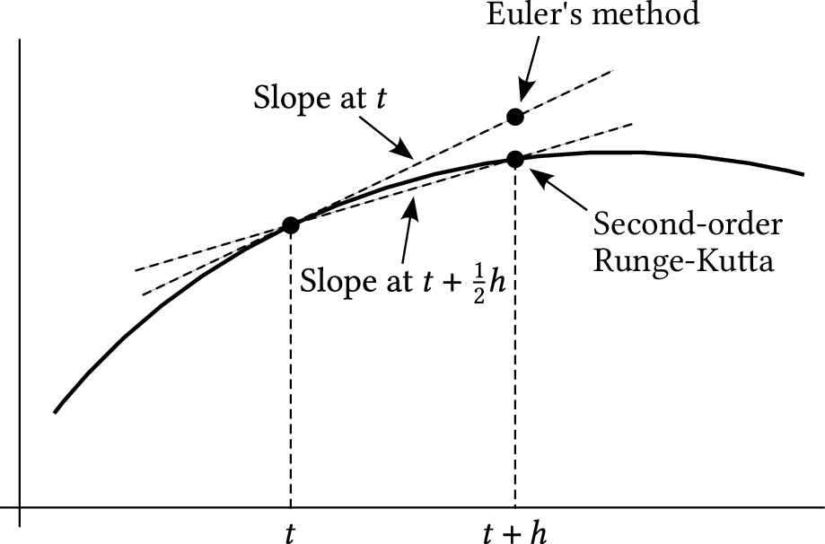
| PDF | PNG | 8.2 | Euler's method and 2nd-order RK
|
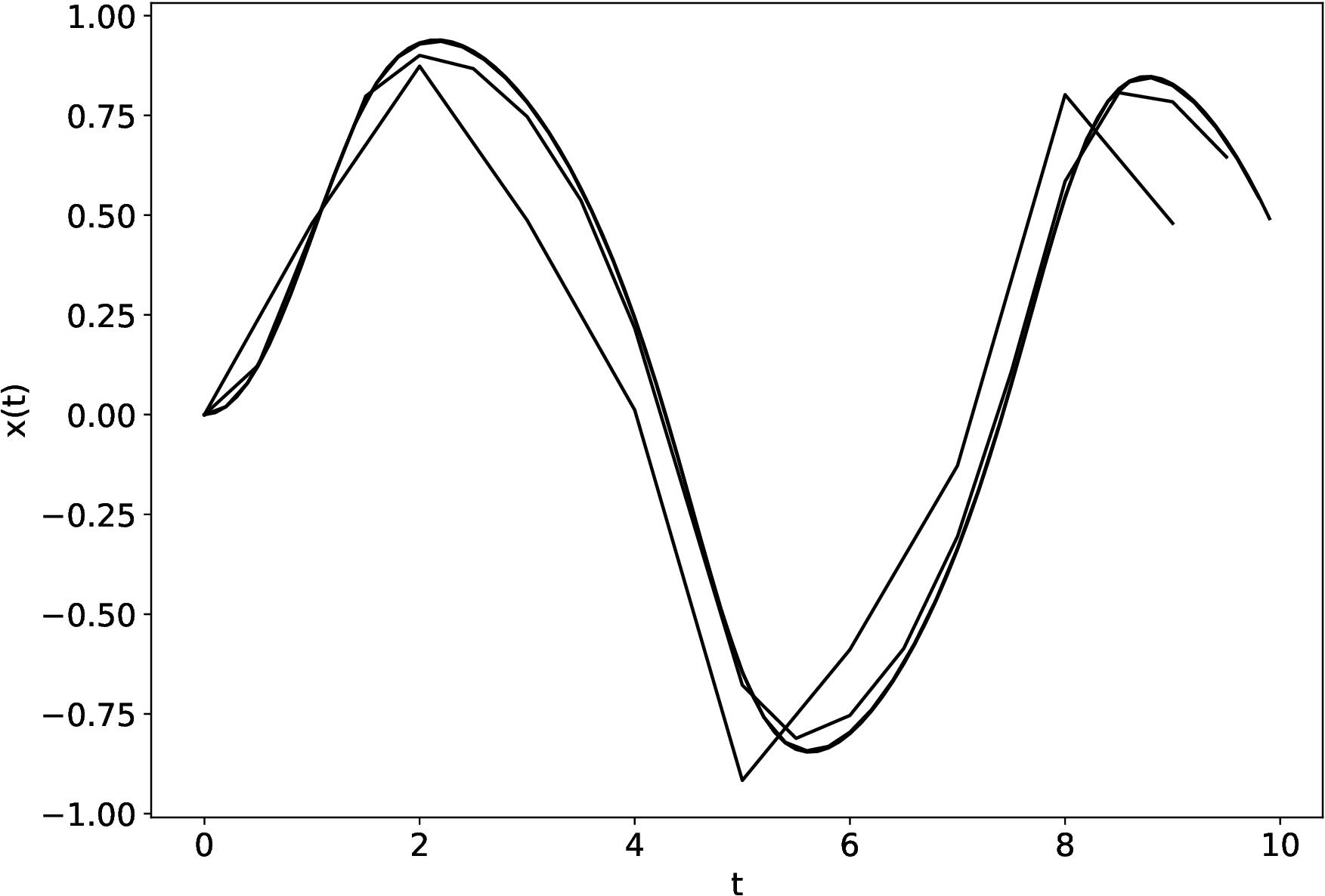
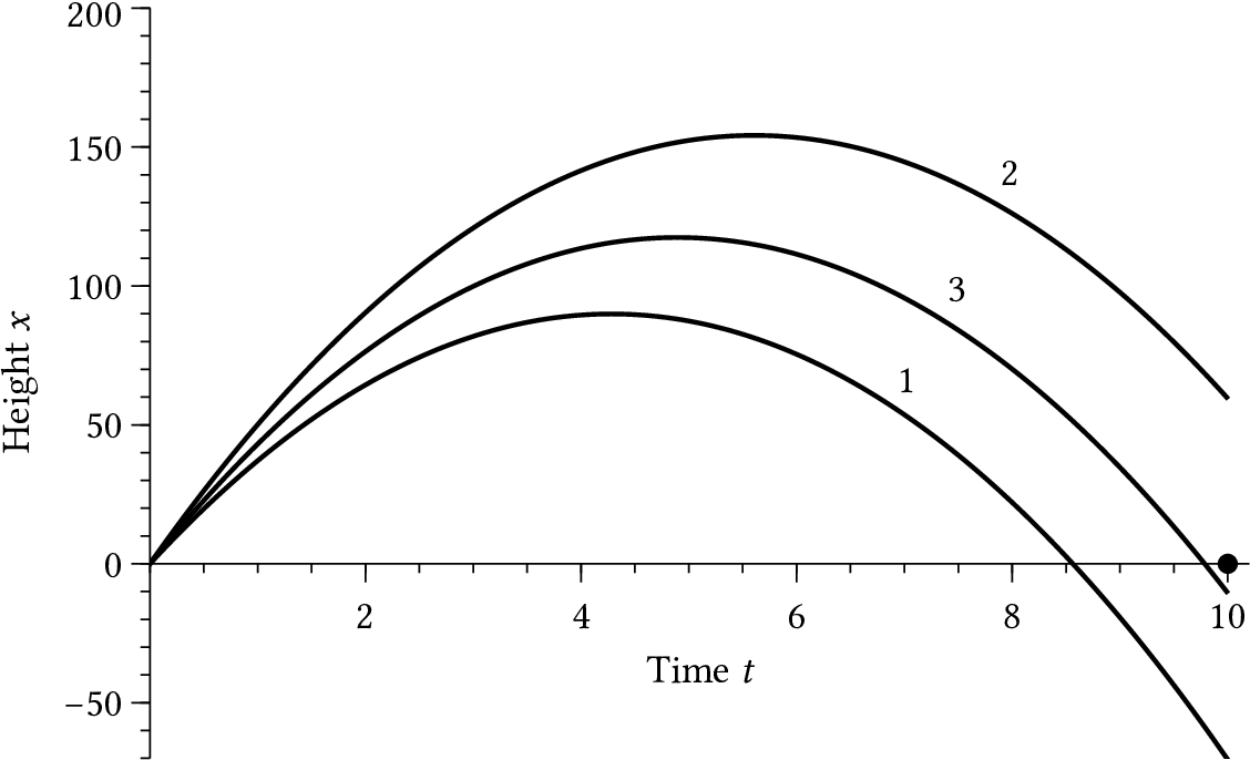
| PDF | PNG | 8.3 | Solutions using 2nd-order RK
|
| PDF | PNG | 8.4 | Solutions using 4th-order RK
|
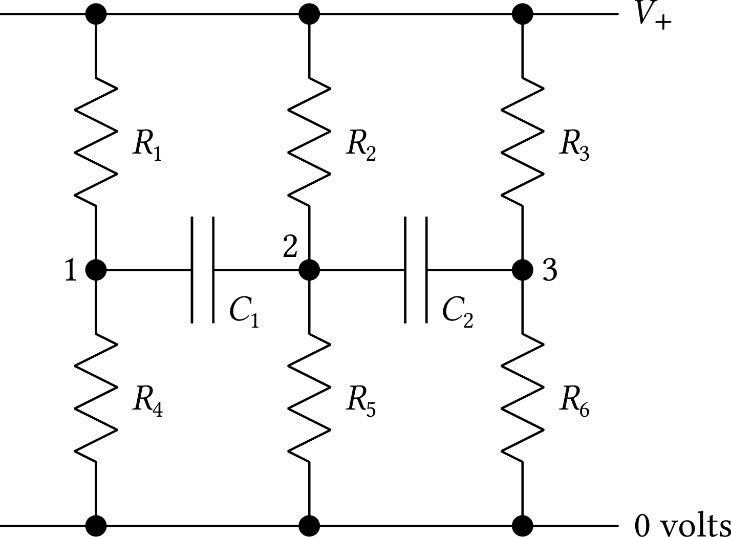
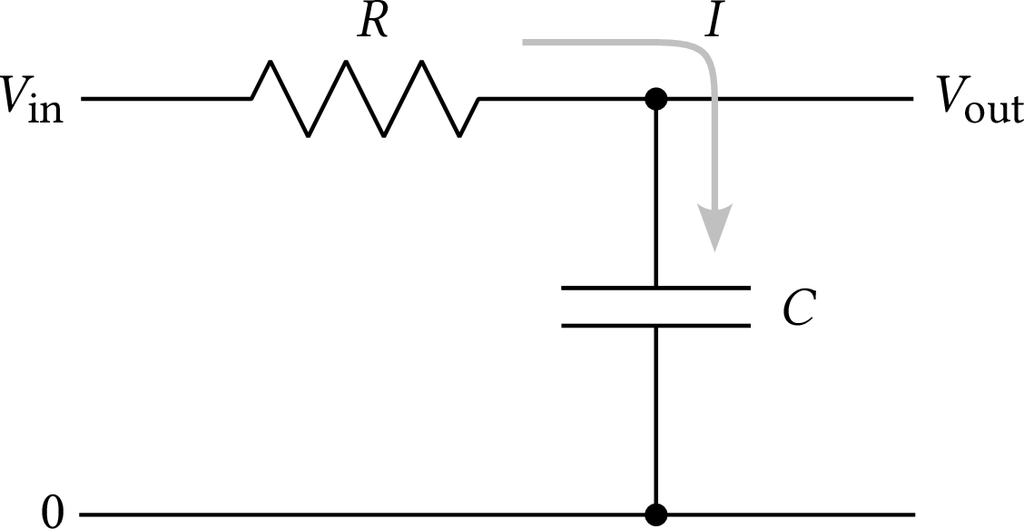
| PDF | PNG | – | Low-pass filter circuit
|
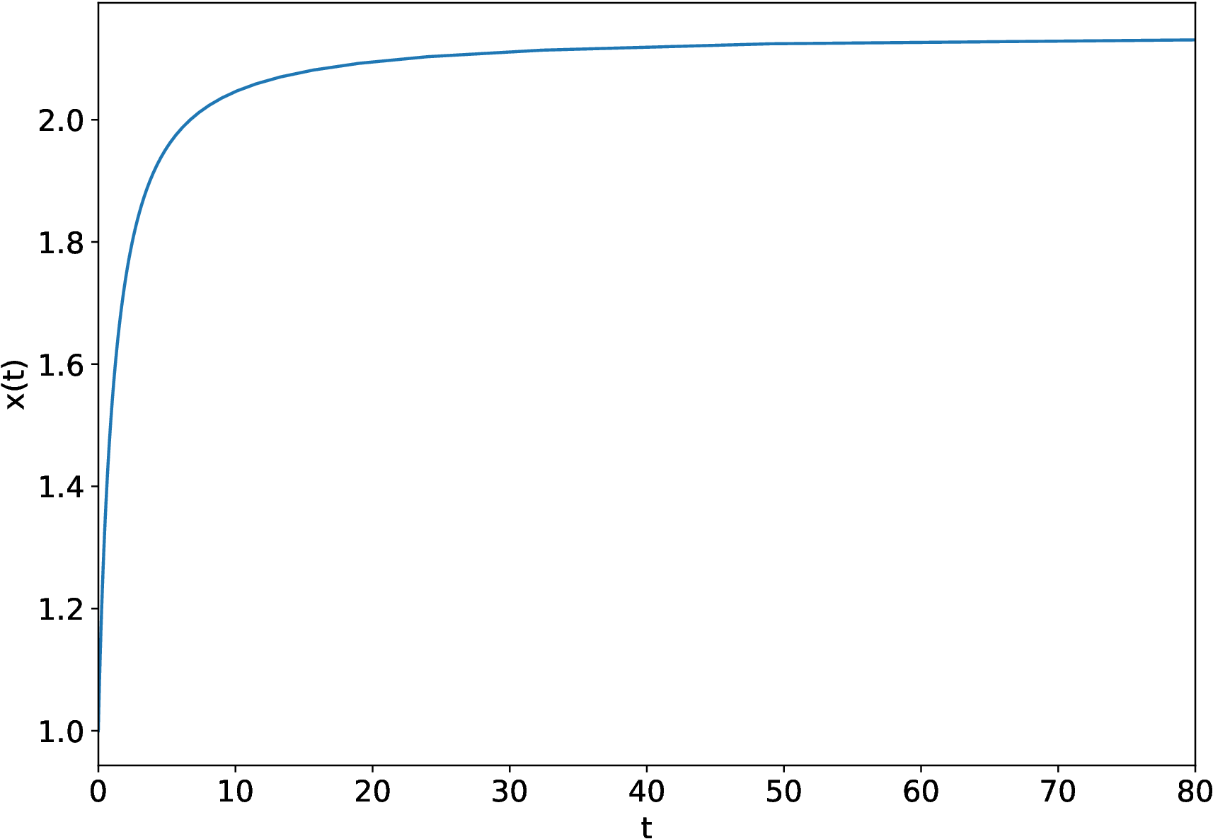
| PDF | PNG | 8.5 | Solution out to infinity
|
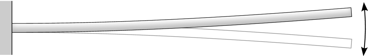
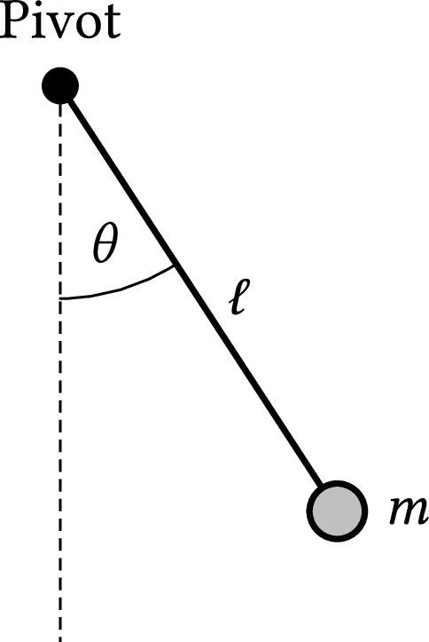
| PDF | PNG | – | Pendulum
|
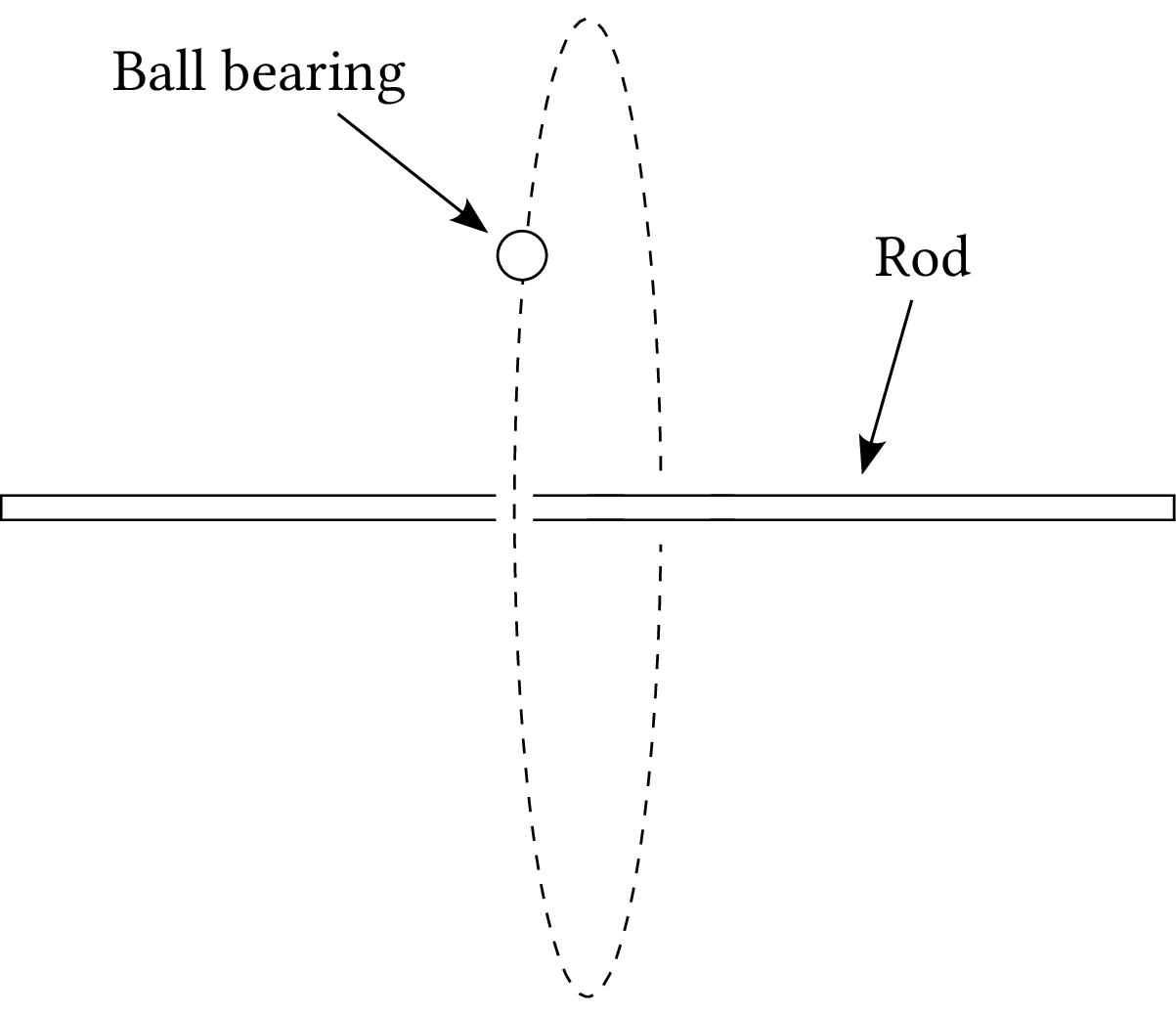
| PDF | PNG | – | Ball bearing and rod
|
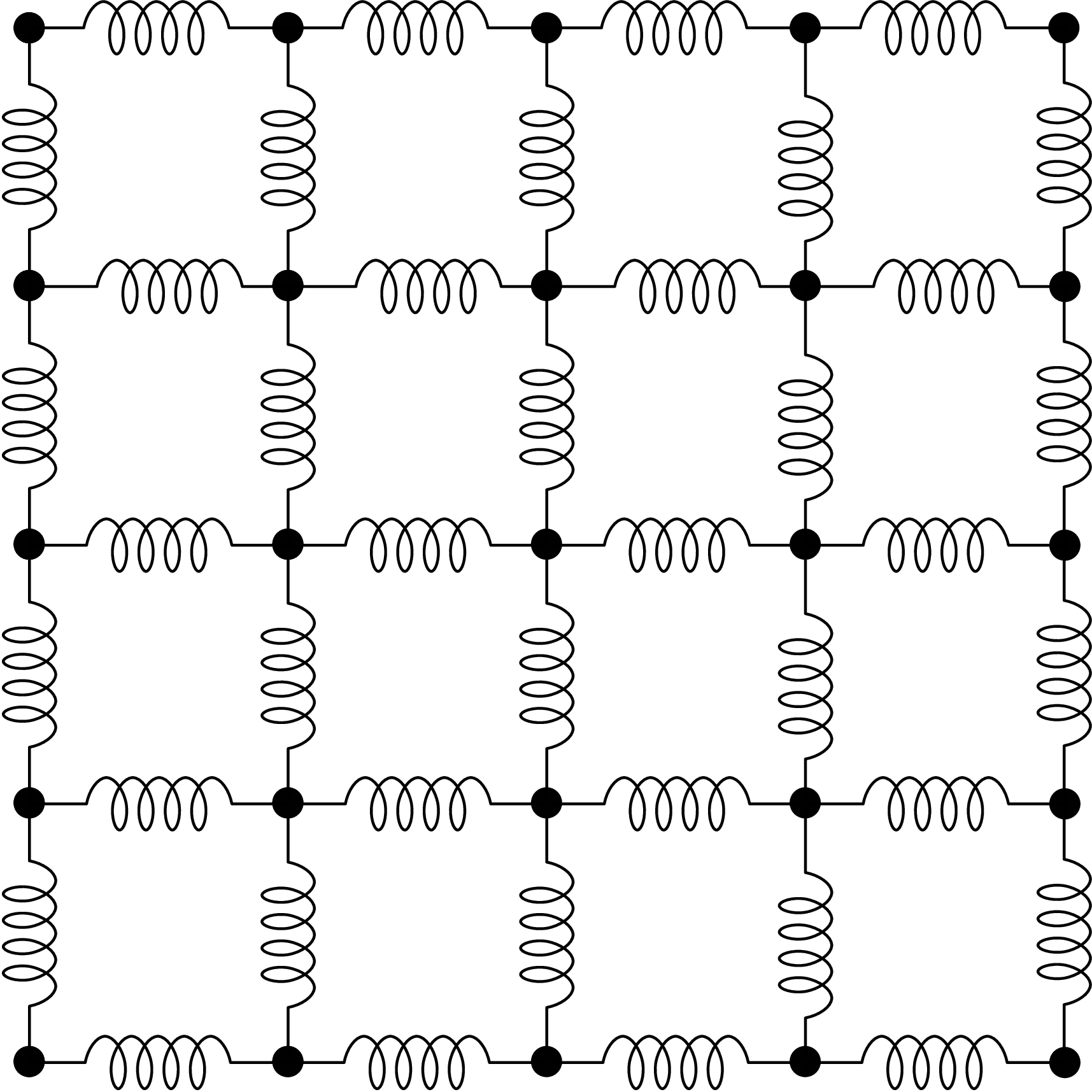
| PDF | PNG | – | Masses and springs
|
| PDF | PNG | 8.6 | Adaptive step sizes
|
| PDF | PNG | 8.7 | Adaptive step size method
|
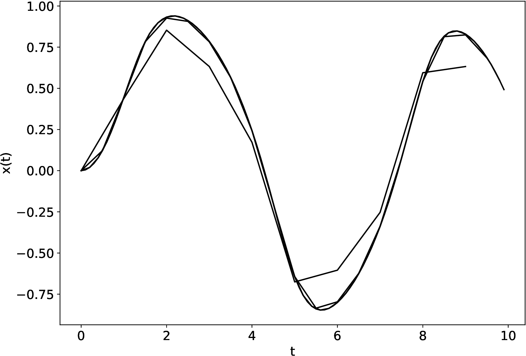
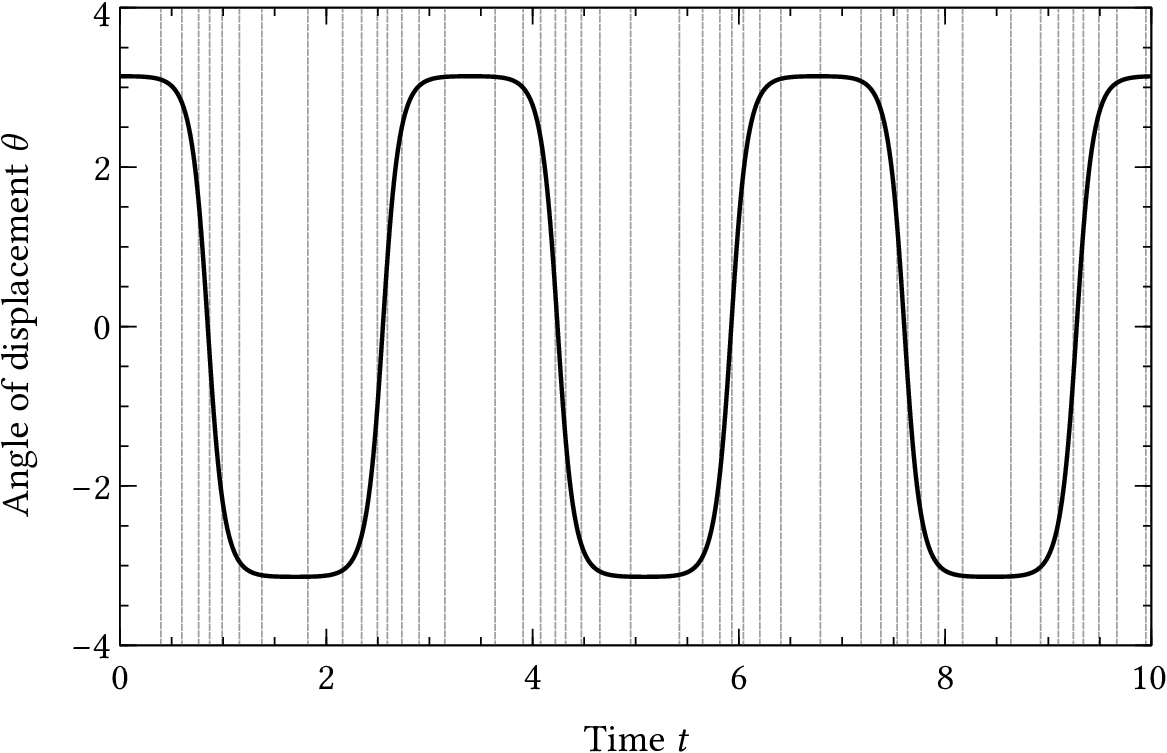
| PDF | PNG | 8.8 | Motion of nonlinear pendulum
|
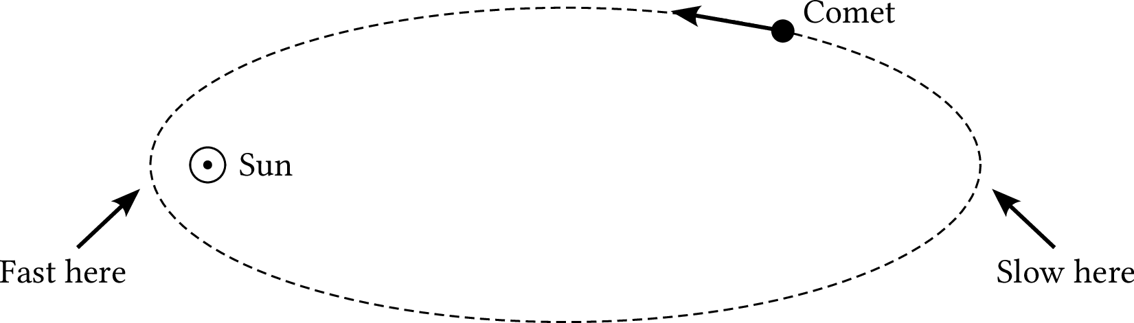
| PDF | PNG | – | Orbit of a comet
|
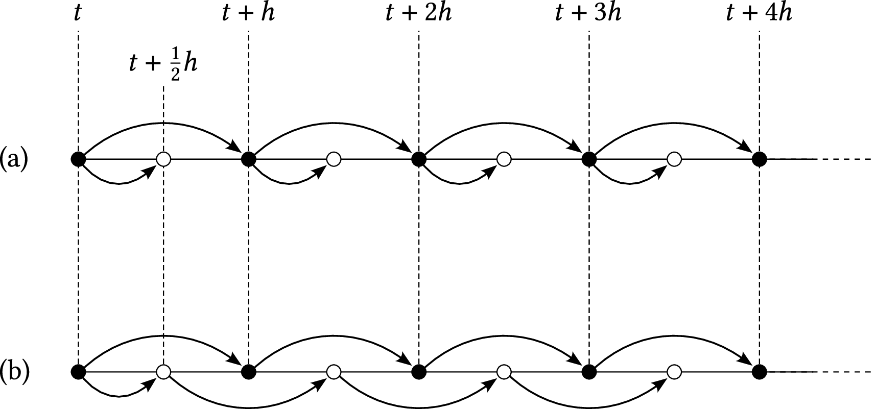
| PDF | PNG | 8.9 | 2nd-order RK and leapfrog method
|
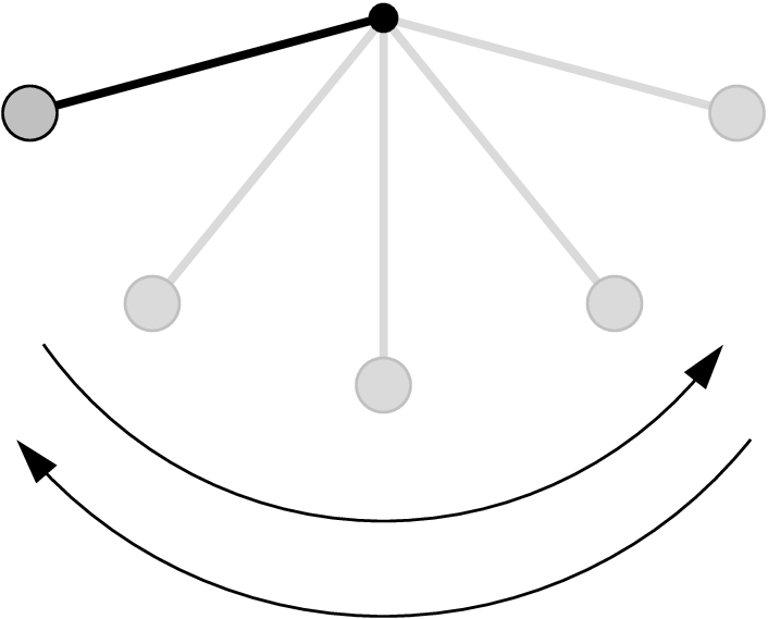
| PDF | PNG | – | One swing of a pendulum
|
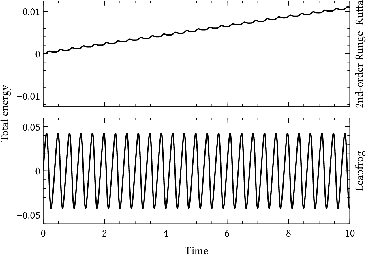
| PDF | PNG | 8.10 | Total energy of pendulum
|
| PDF | PNG | – | Adaptive step sizes
|
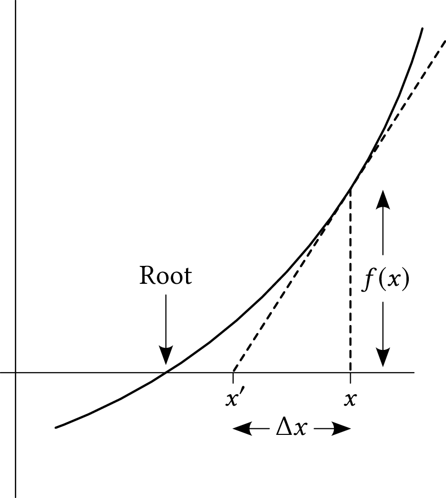
| PDF | PNG | 8.11 | The shooting method
|
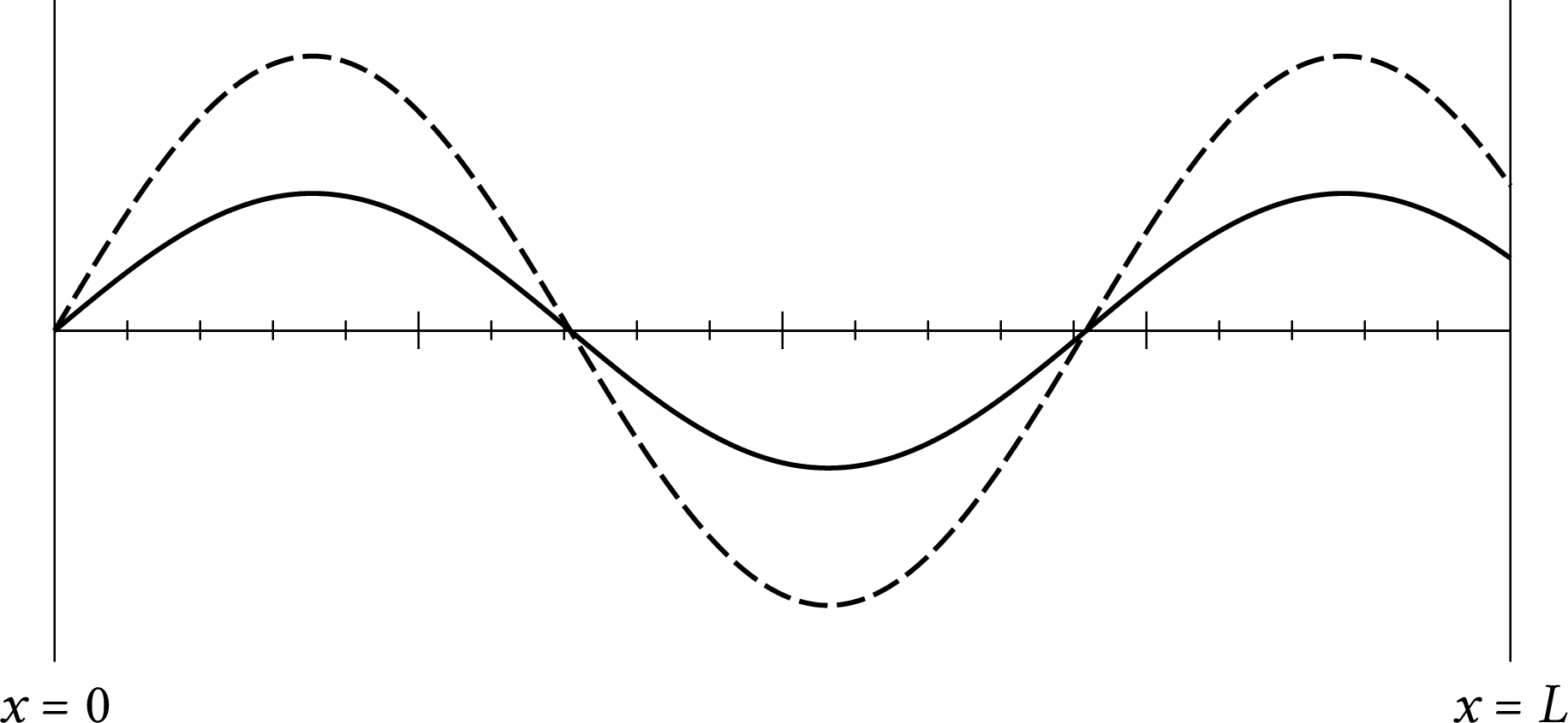
| PDF | PNG | 8.12 | Schrodinger equation in square well
|
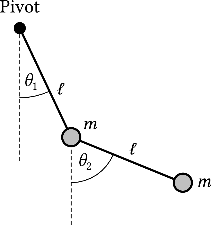
| PDF | PNG | – | Double pendulum
|
Chapter 9: Partial differential equations
| Format | Figure | Description |
|---|
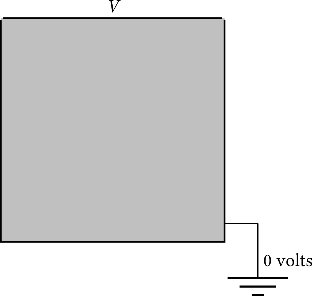
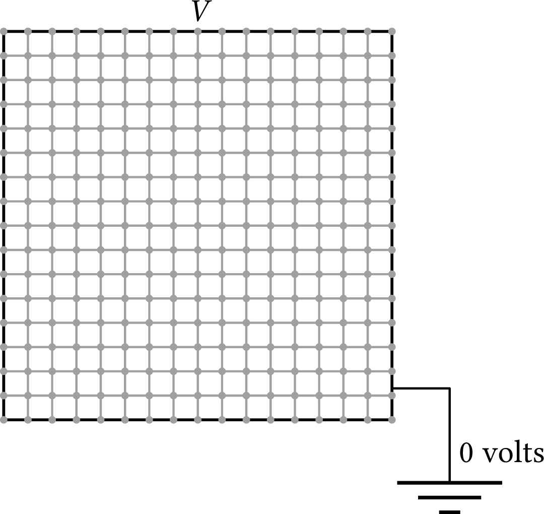
| PDF | PNG | 9.1 | Simple electrostatics problem
|
| PDF | PNG | 9.2 | A square grid
|
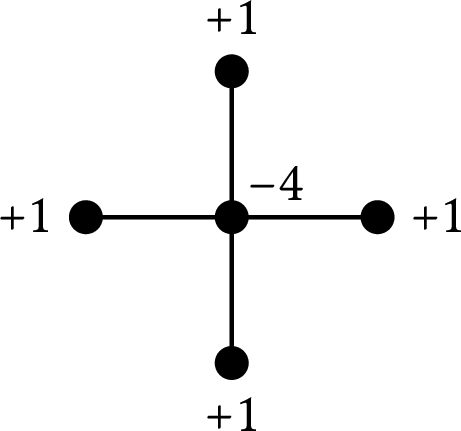
| PDF | PNG | – | Laplacian diagram
|
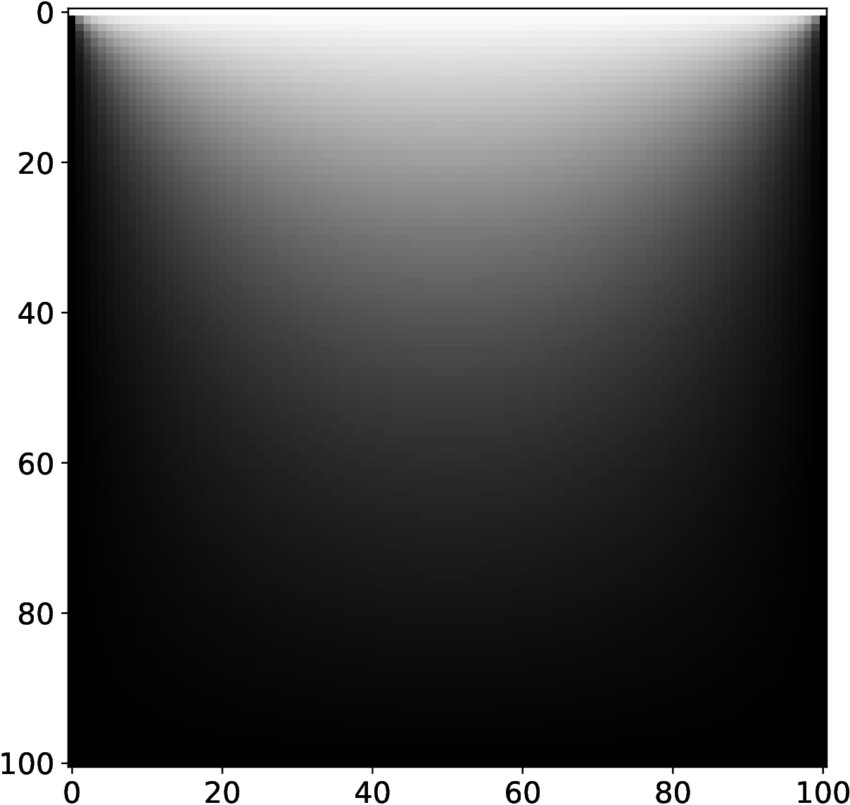
| PDF | PNG | 9.3 | Solution of Laplace equation
|
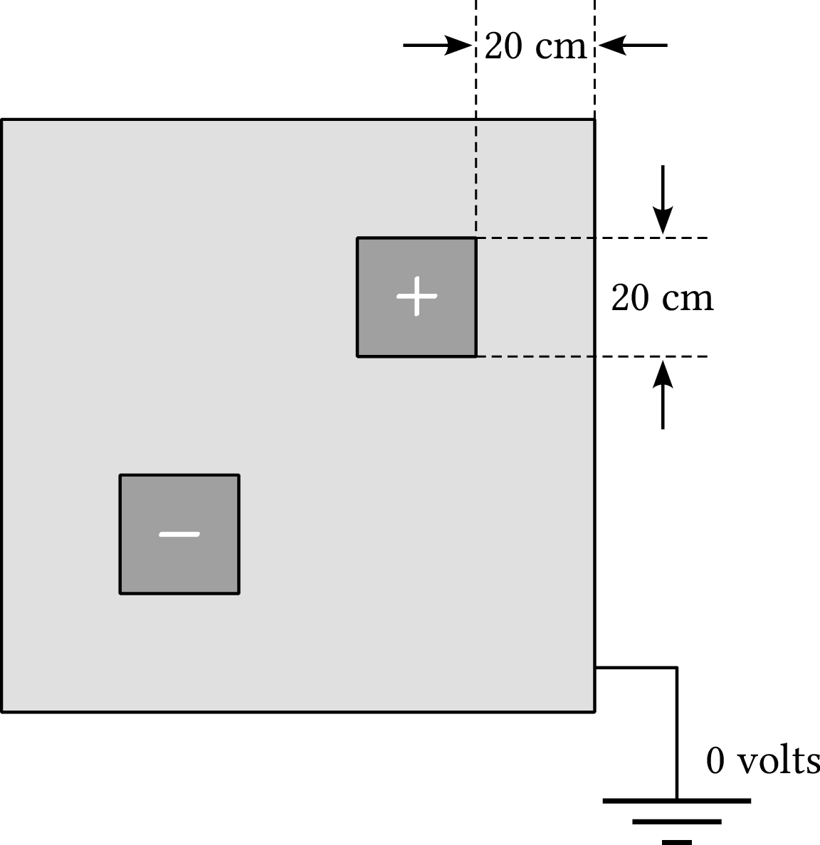
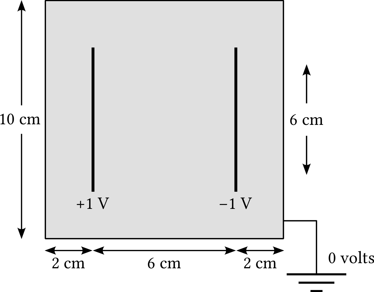
| PDF | PNG | 9.4 | More complicated electrostatics problem
|
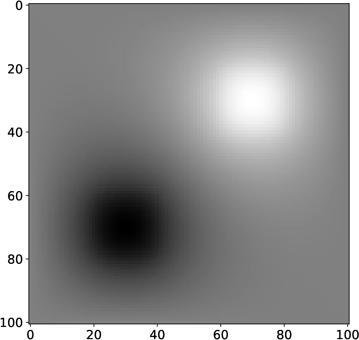
| PDF | PNG | 9.5 | Solution of Poisson equation
|
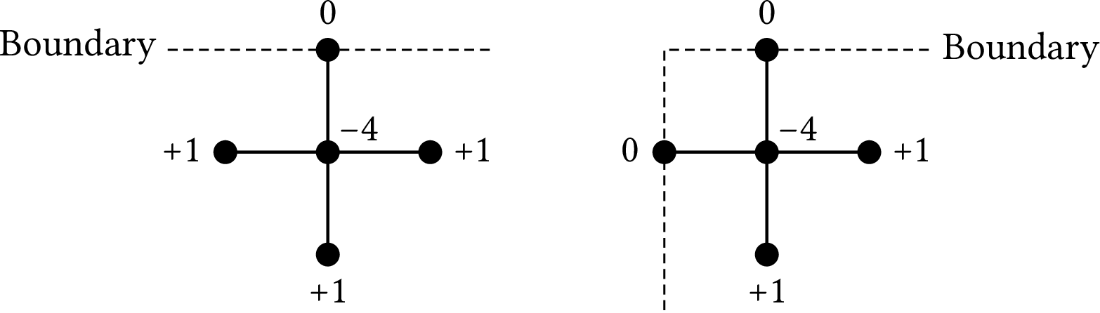
| PDF | PNG | – | Dirichlet boundary conditions
|
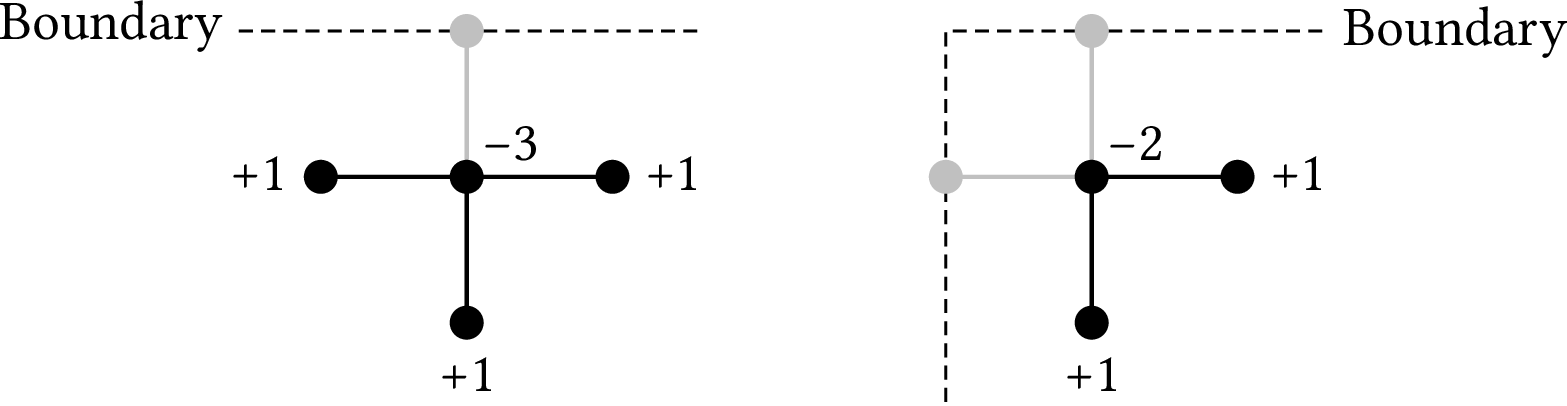
| PDF | PNG | – | Neumann boundary conditions
|
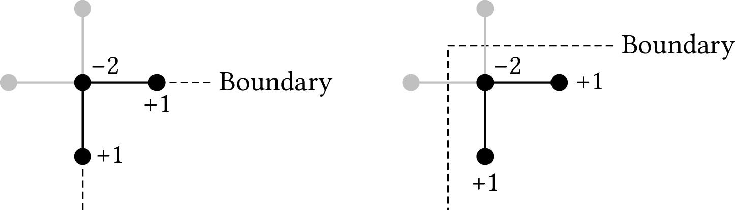
| PDF | PNG | – | Variant boundary conditions
|
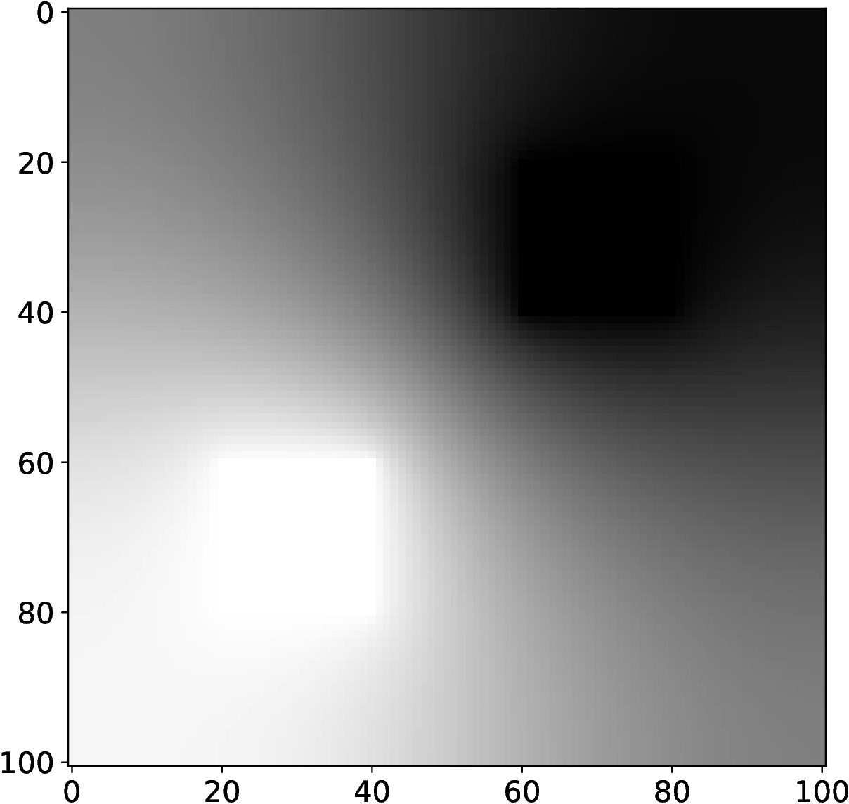
| PDF | PNG | 9.6 | Solution of heat equation
|
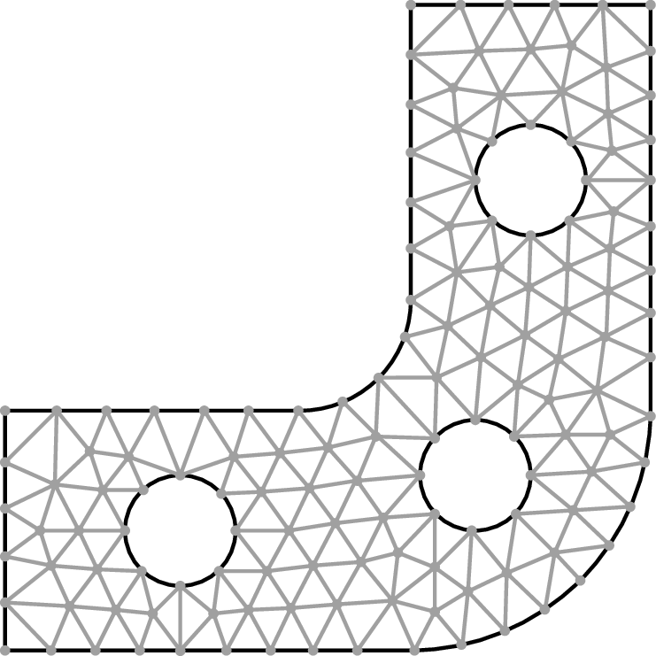
| PDF | PNG | 9.7a | Triangulation with three holes
|
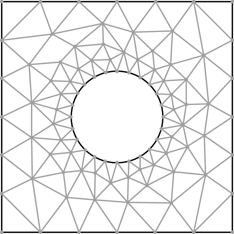
| PDF | PNG | 9.7b | Triangulation with one hole
|
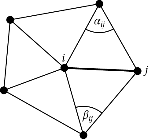
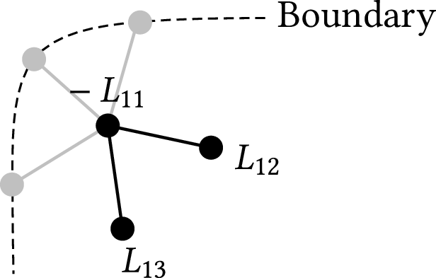
| PDF | PNG | 9.8 | Laplacian on a triangulation
|
| PDF | PNG | – | Boundary of a triangulation
|
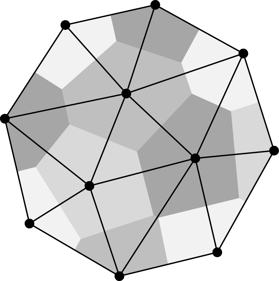
| PDF | PNG | 9.9 | Delaunay triangulation
|
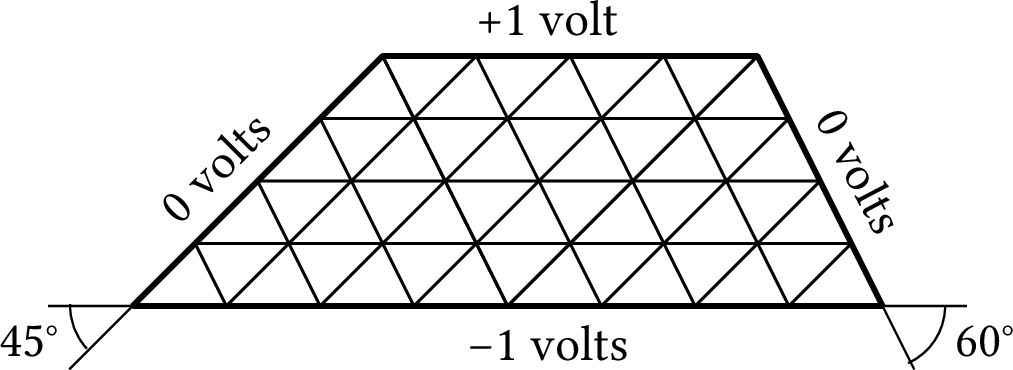
| PDF | PNG | – | Laplace equation on non-square grid
|
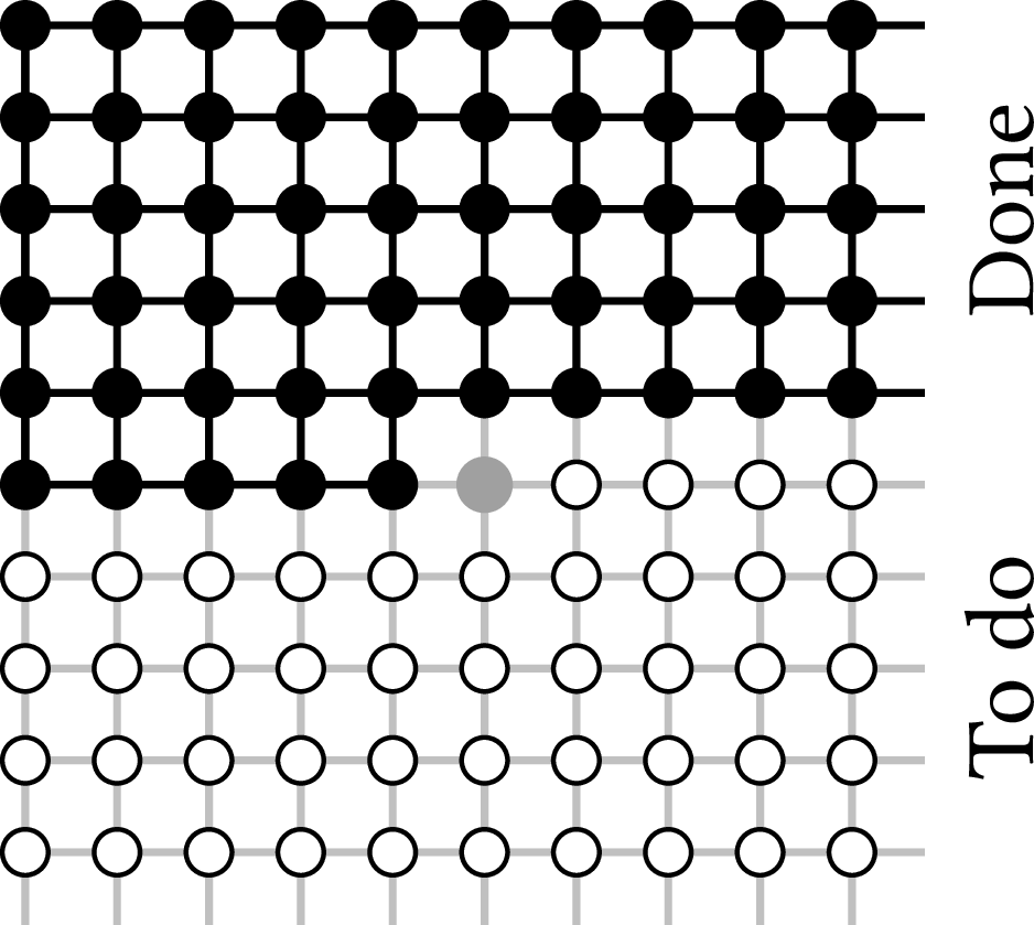
| PDF | PNG | – | The Gauss-Seidel method
|
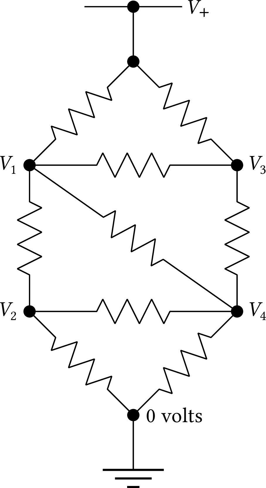
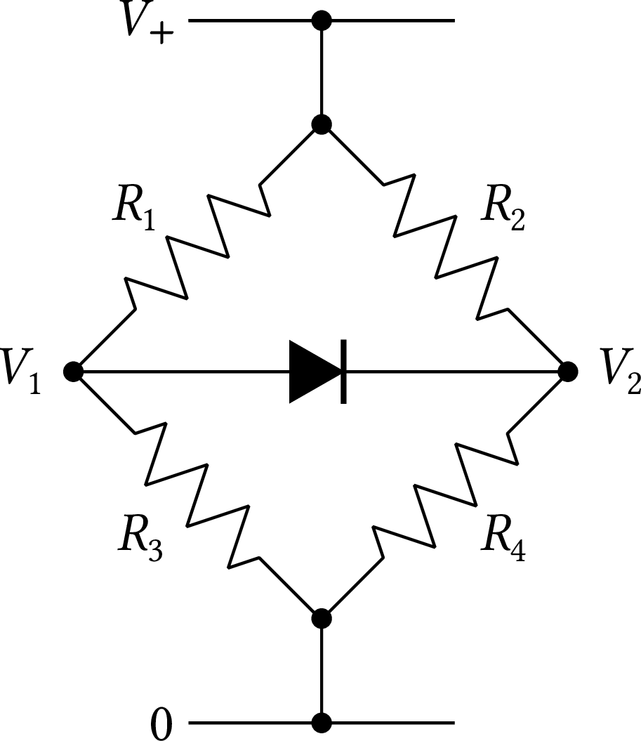
| PDF | PNG | – | Model of a capacitor
|
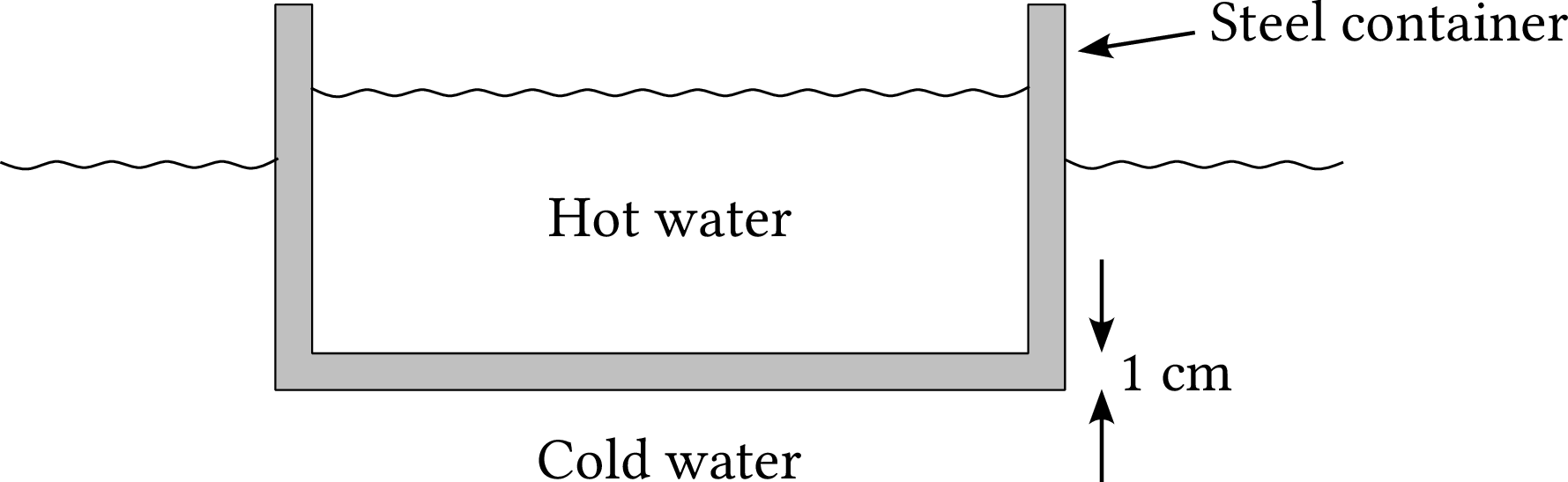
| PDF | PNG | – | Heat flow problem
|
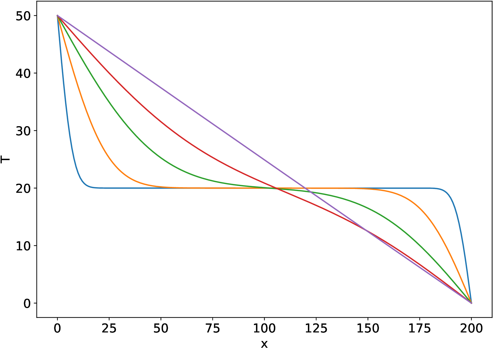
| PDF | PNG | 9.10 | Solution of heat flow problem
|
| PDF | PNG | 9.11a | Instability in FTCS solution 1
|
| PDF | PNG | 9.11b | Instability in FTCS solution 2
|
| PDF | PNG | 9.11c | Instability in FTCS solution 3
|
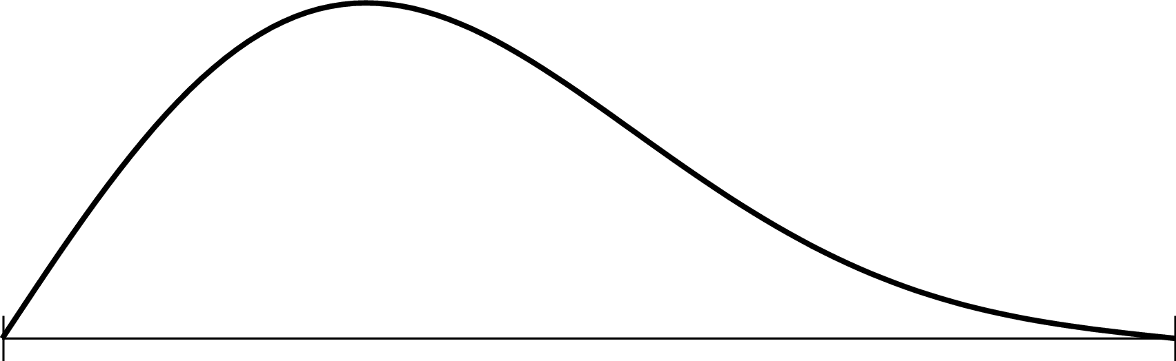
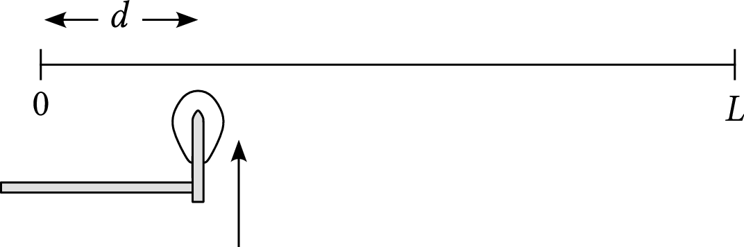
| PDF | PNG | – | Piano hammer and string
|
Chapter 10: Random processes and Monte Carlo methods
| Format | Figure | Description |
|---|
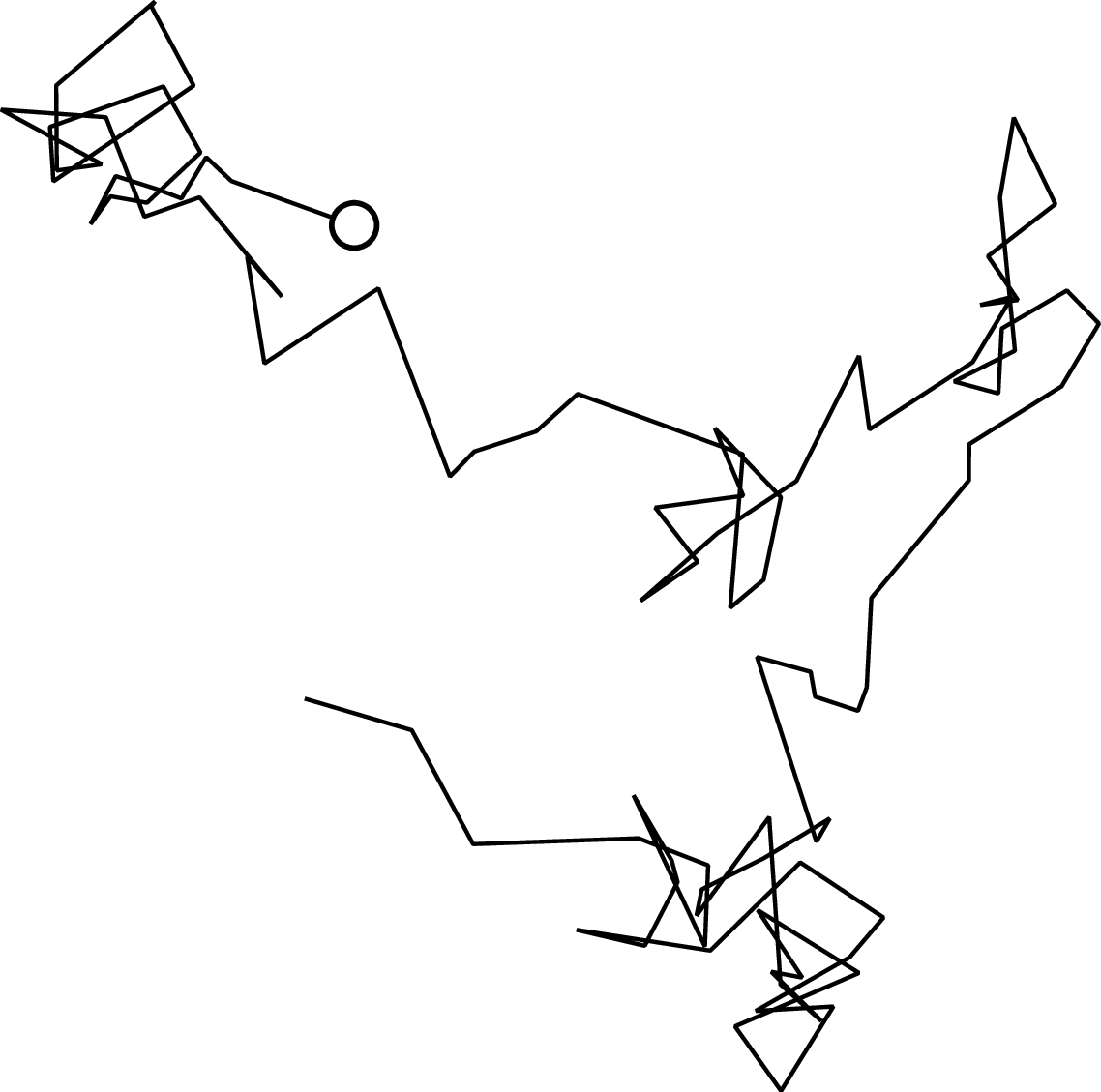
| PDF | PNG | – | Brownian motion
|
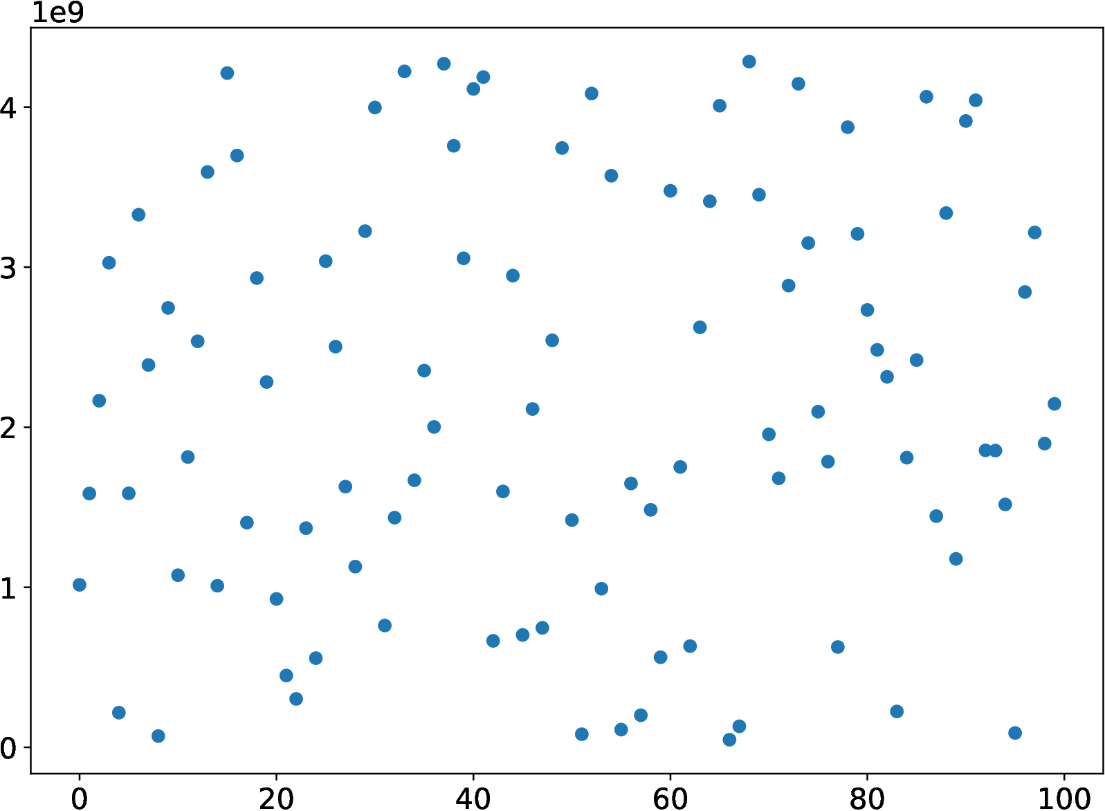
| PDF | PNG | 10.1 | Linear congruential generator
|
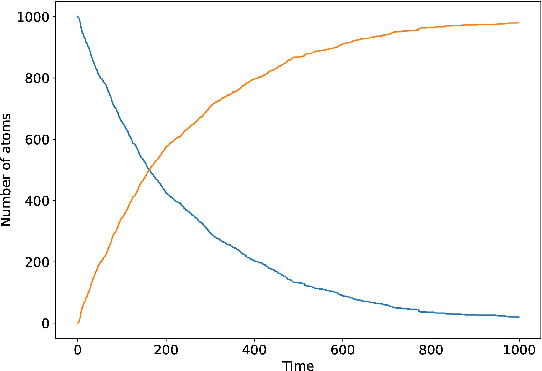
| PDF | PNG | 10.2 | Radioactive decay
|
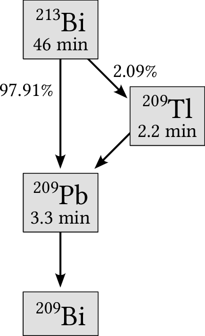
| PDF | PNG | – | Decay chain
|
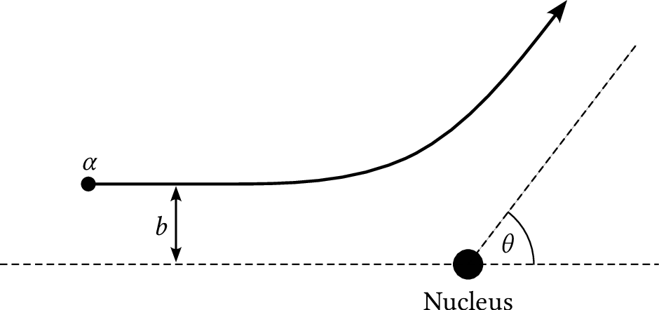
| PDF | PNG | 10.3 | Rutherford scattering
|
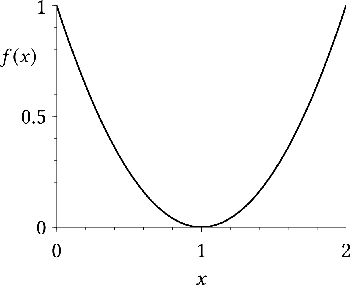
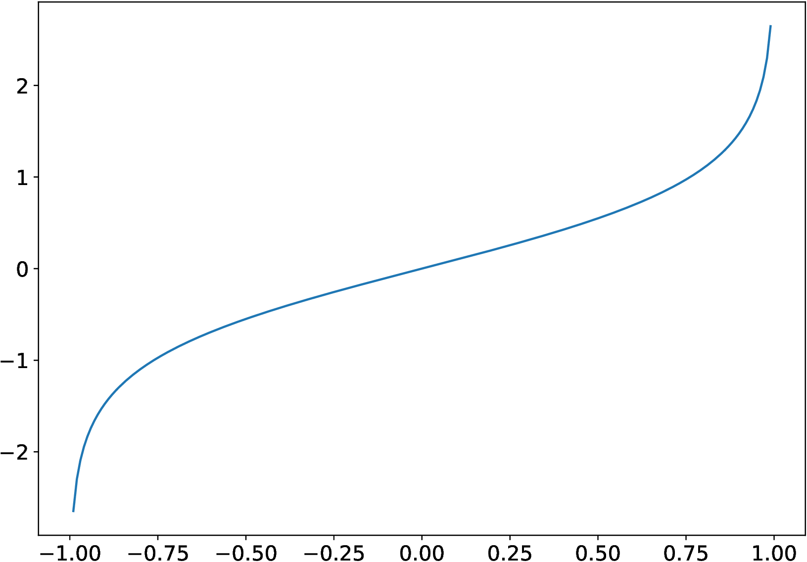
| PDF | PNG | 10.4 | A pathological function
|
| PDF | PNG | – | Area of a circle
|
| PDF | PNG | 10.5 | Integrand
|
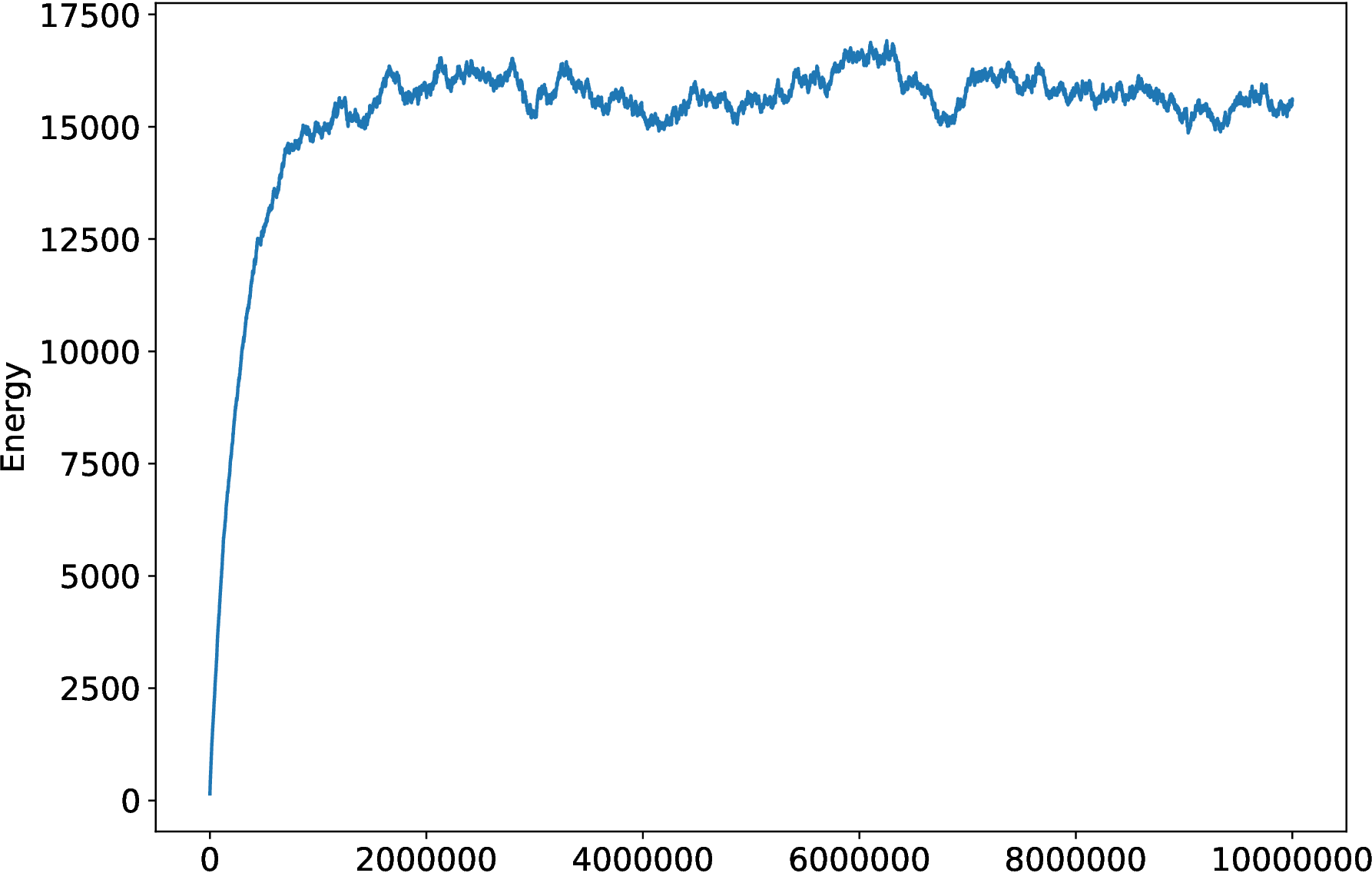
| PDF | PNG | 10.6 | Internal energy of ideal gas
|
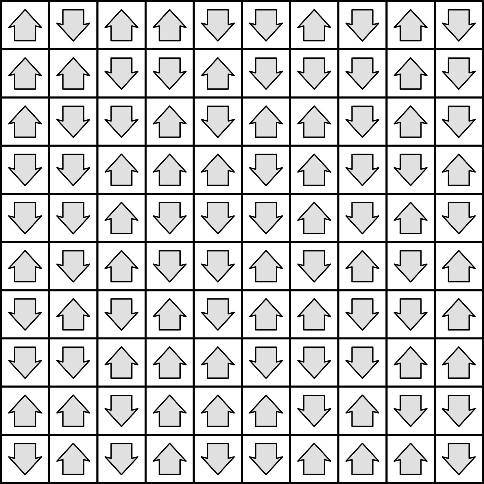
| PDF | PNG | – | The Ising model
|
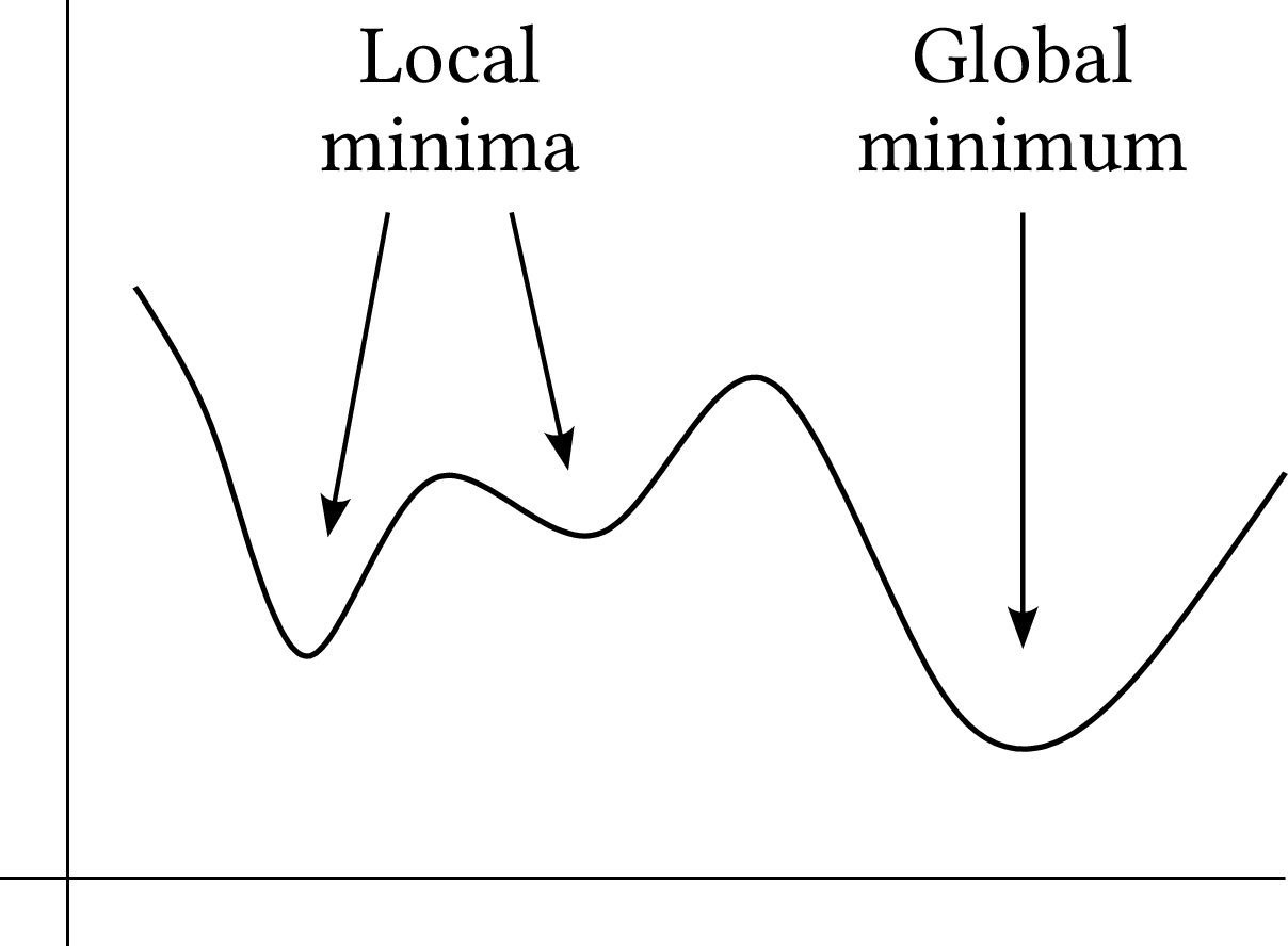
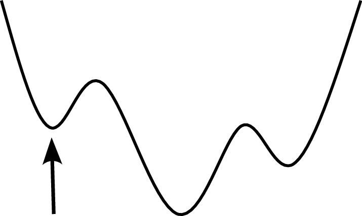
| PDF | PNG | – | Local minimum
|
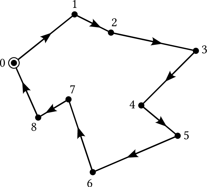
| PDF | PNG | 10.7 | The traveling salesman problem
|
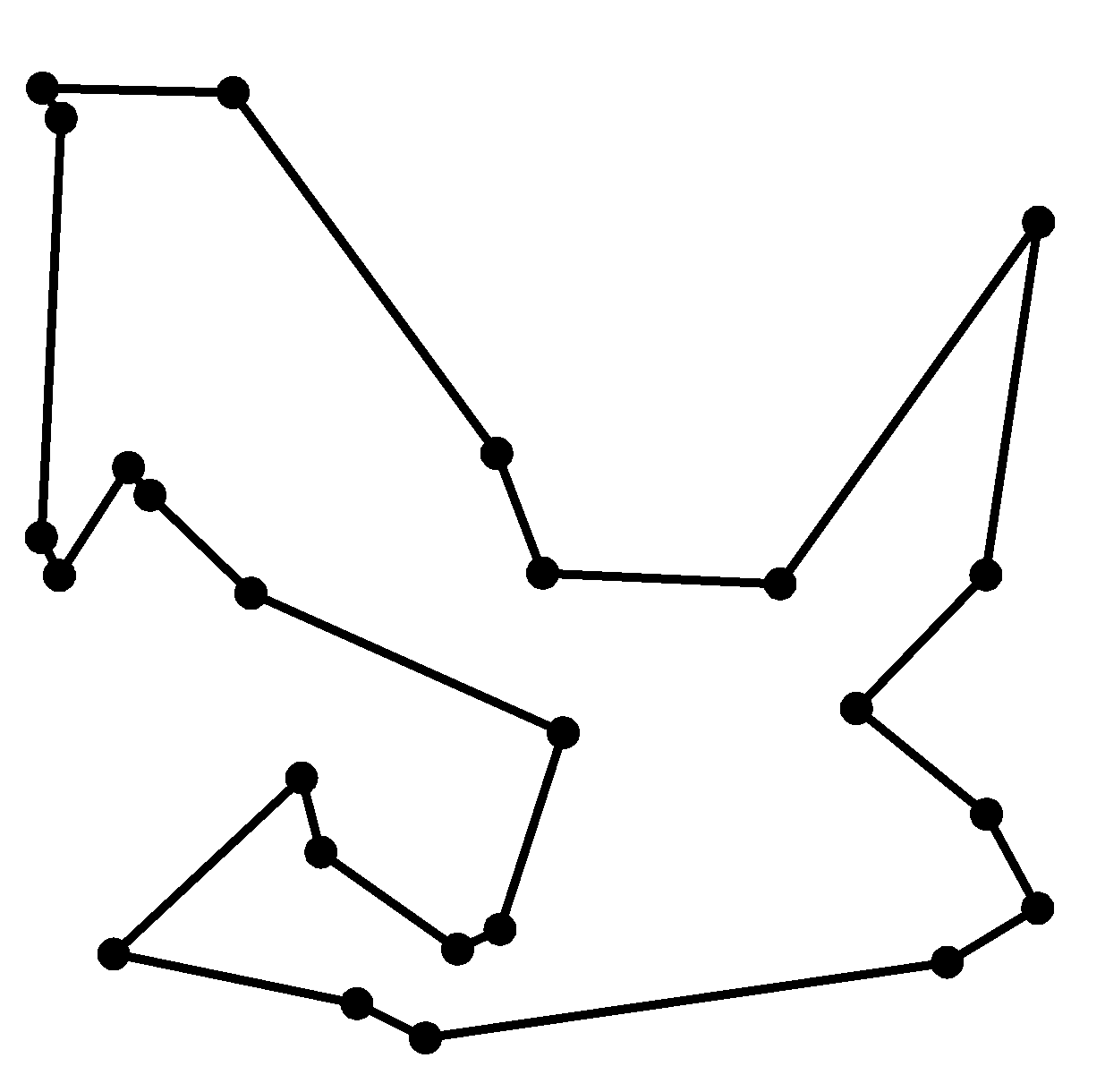
| – | PNG | 10.8a | Solution 1 of the traveling salesman problem
|
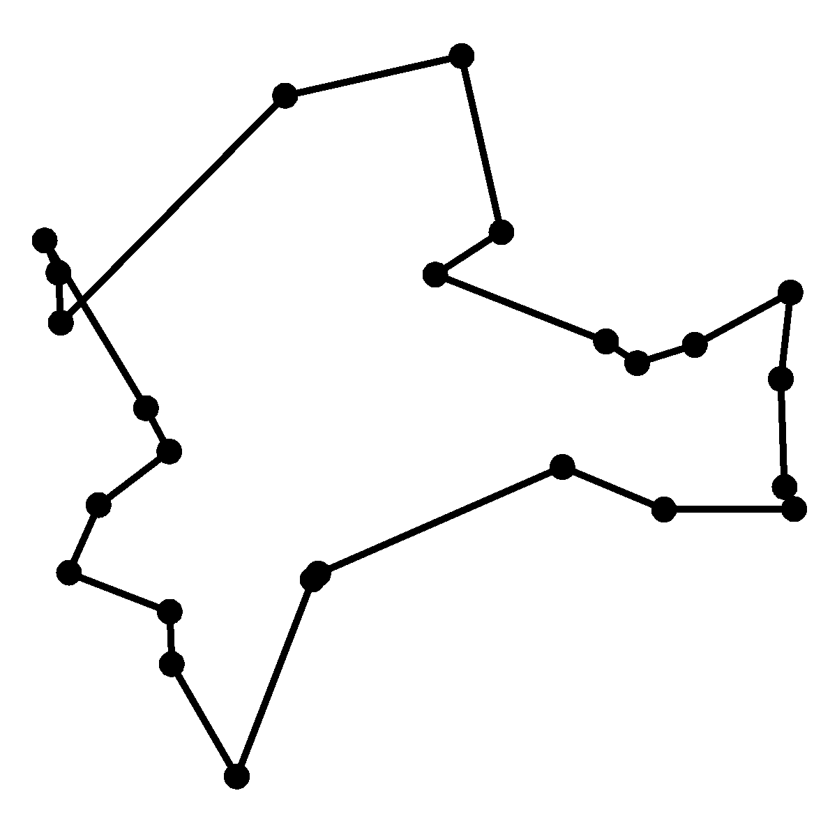
| – | PNG | 10.8b | Solution 2 of the traveling salesman problem
|
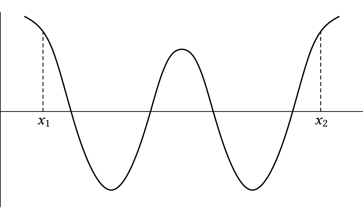
| PDF | PNG | 10.9 | Function from Exercise 10.11
|
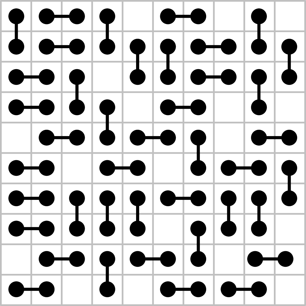
| PDF | PNG | – | Dimer covering
|
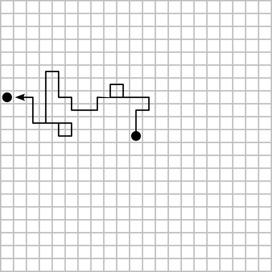
| PDF | PNG | 10.10 | Diffusion-limited aggregation
|
Chapter 11: Data science
| Format | Figure | Description |
|---|
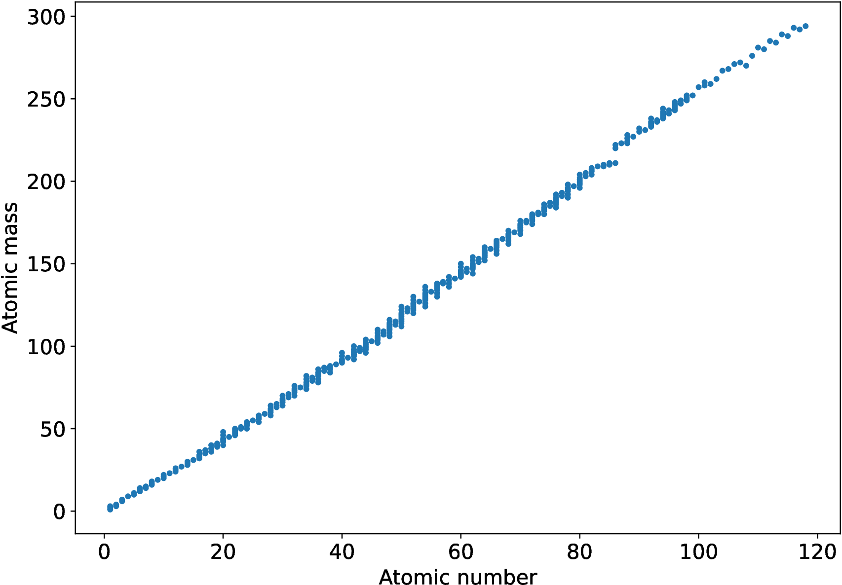
| PDF | PNG | 11.1 | Atomic isotopes
|
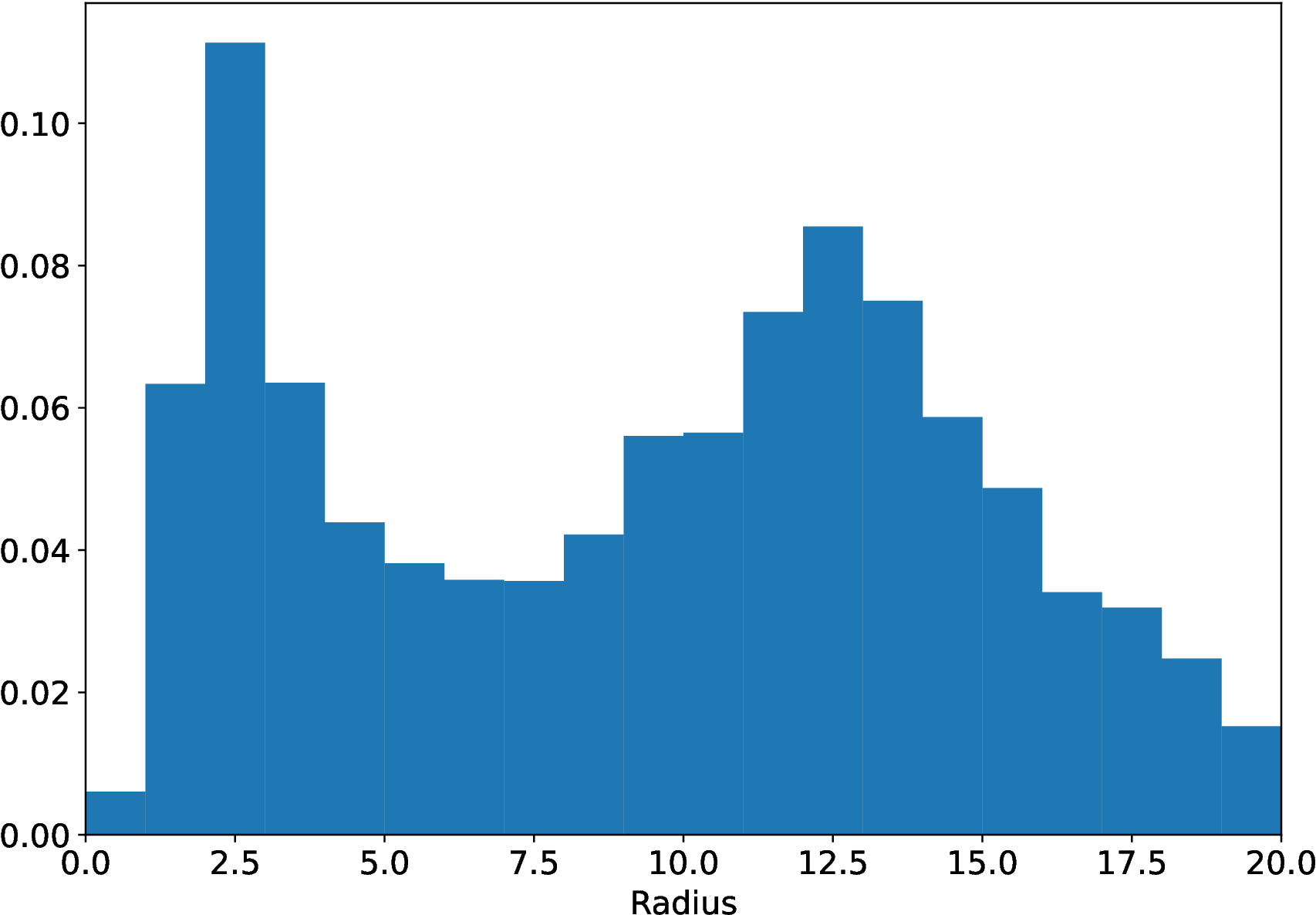
| PDF | PNG | 11.2 | Radii of exoplanets
|
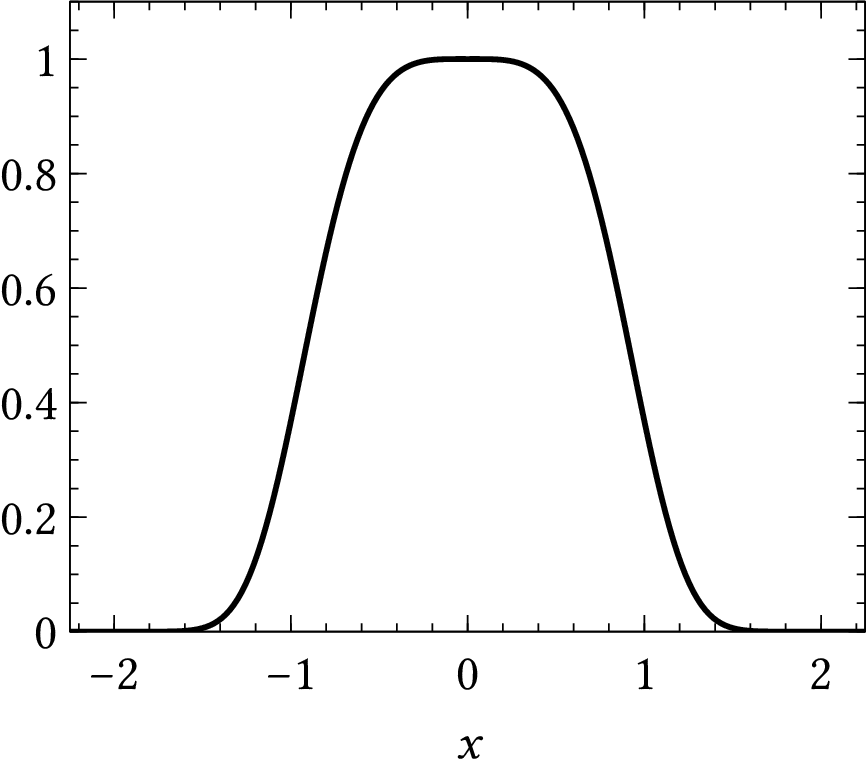
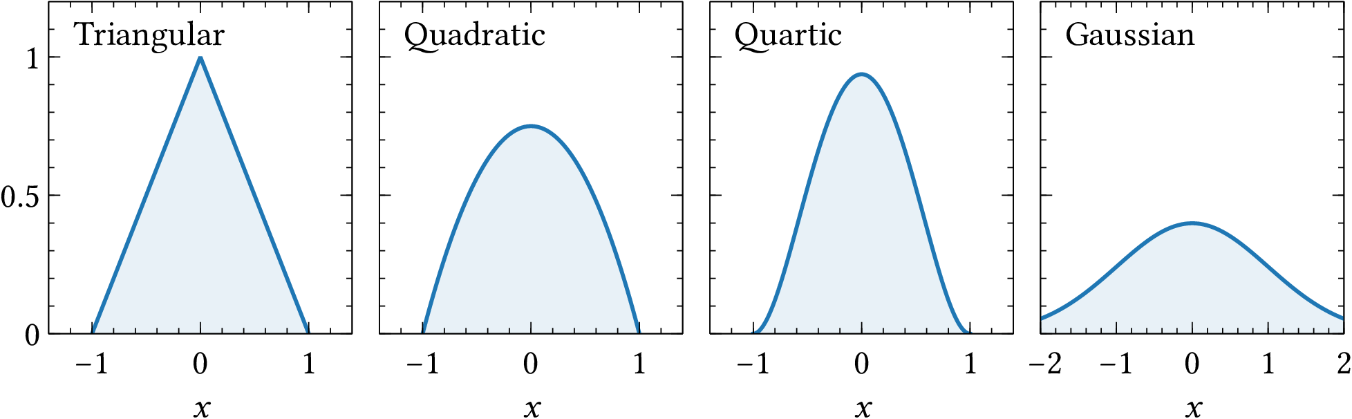
| PDF | PNG | 11.3 | Common kernels
|
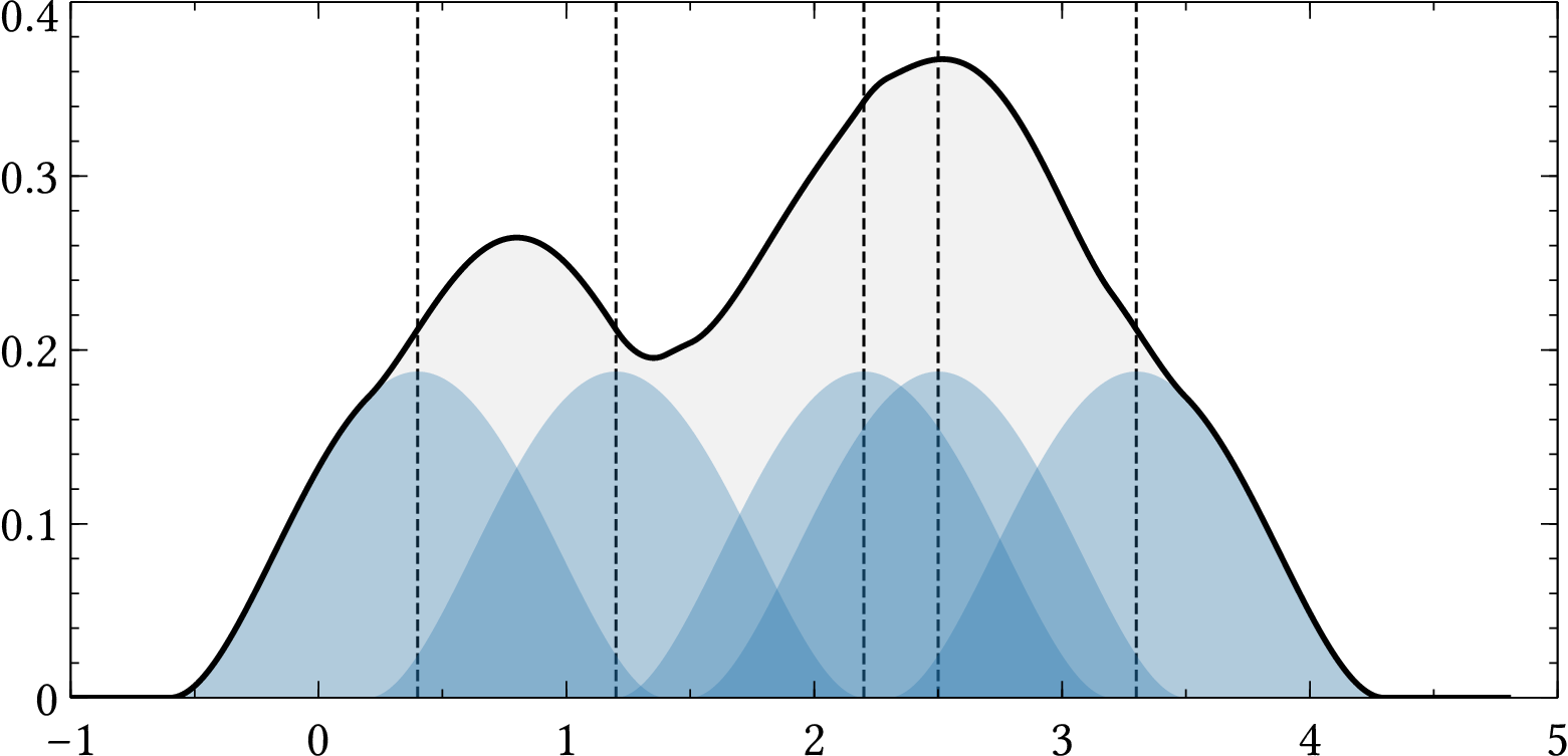
| PDF | PNG | 11.4 | Kernel density estimation
|
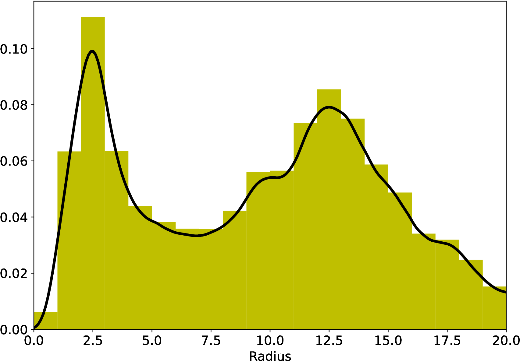
| PDF | PNG | 11.5 | KDE for exoplanet radii
|
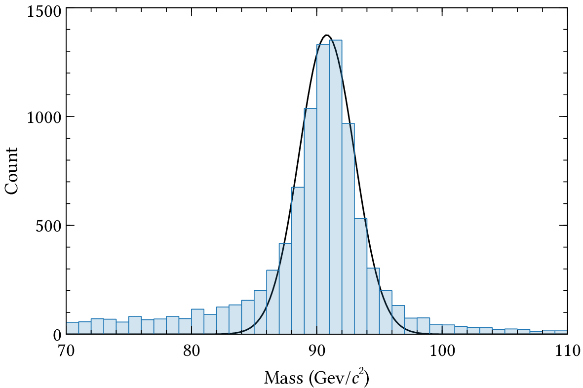
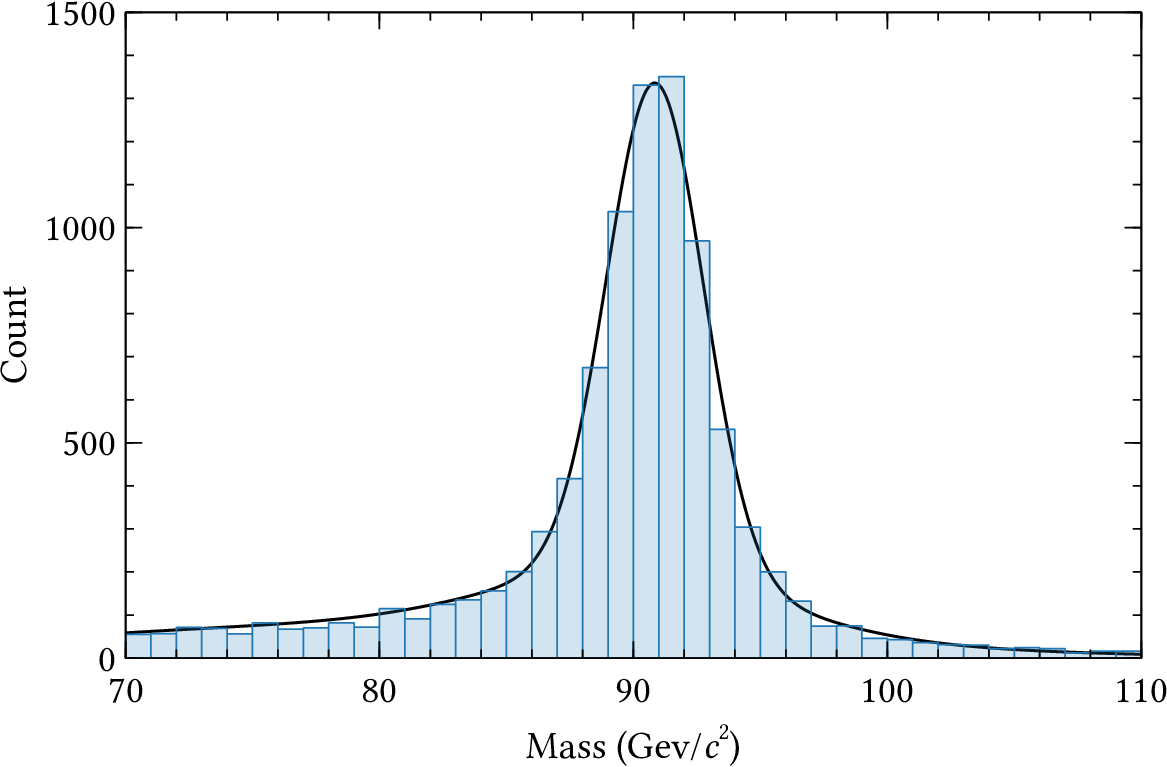
| PDF | PNG | 11.6 | Measurements of Z0 mass
|
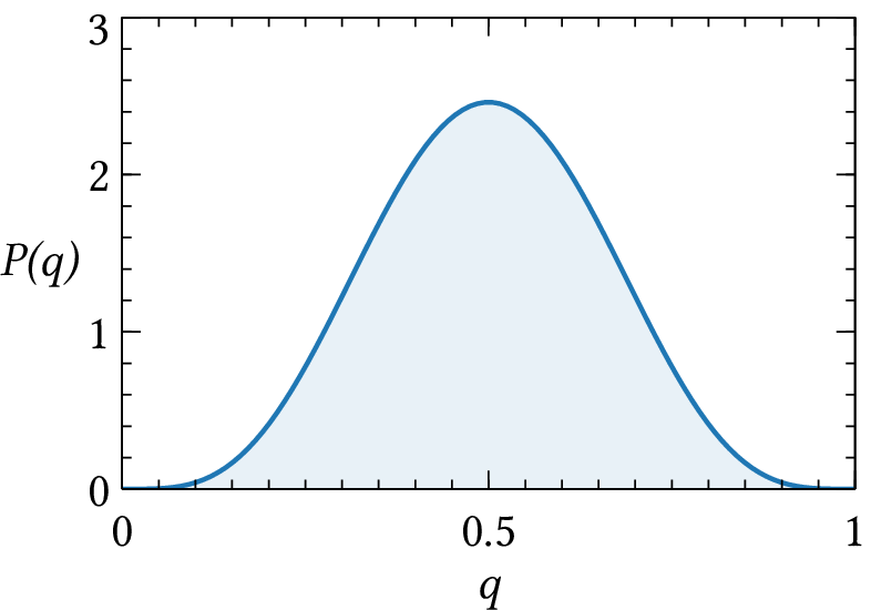
| PDF | PNG | 11.7 | Beta distribution
|
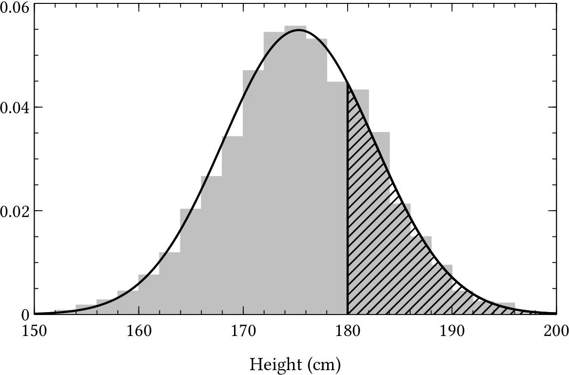
| PDF | PNG | 11.8 | Heights of adult males
|
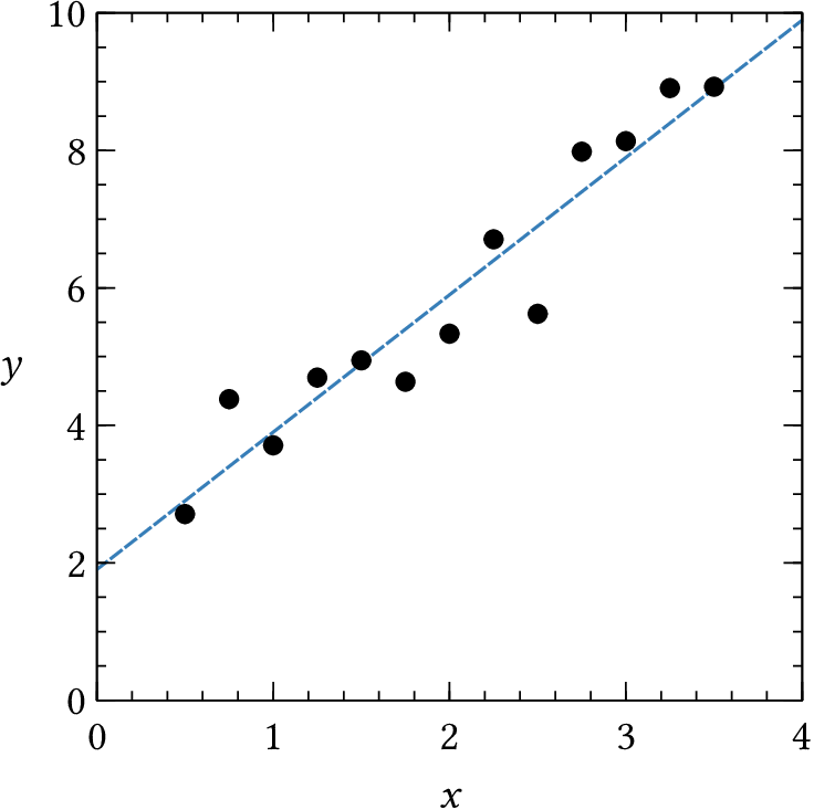
| PDF | PNG | 11.9 | Straight line fit
|
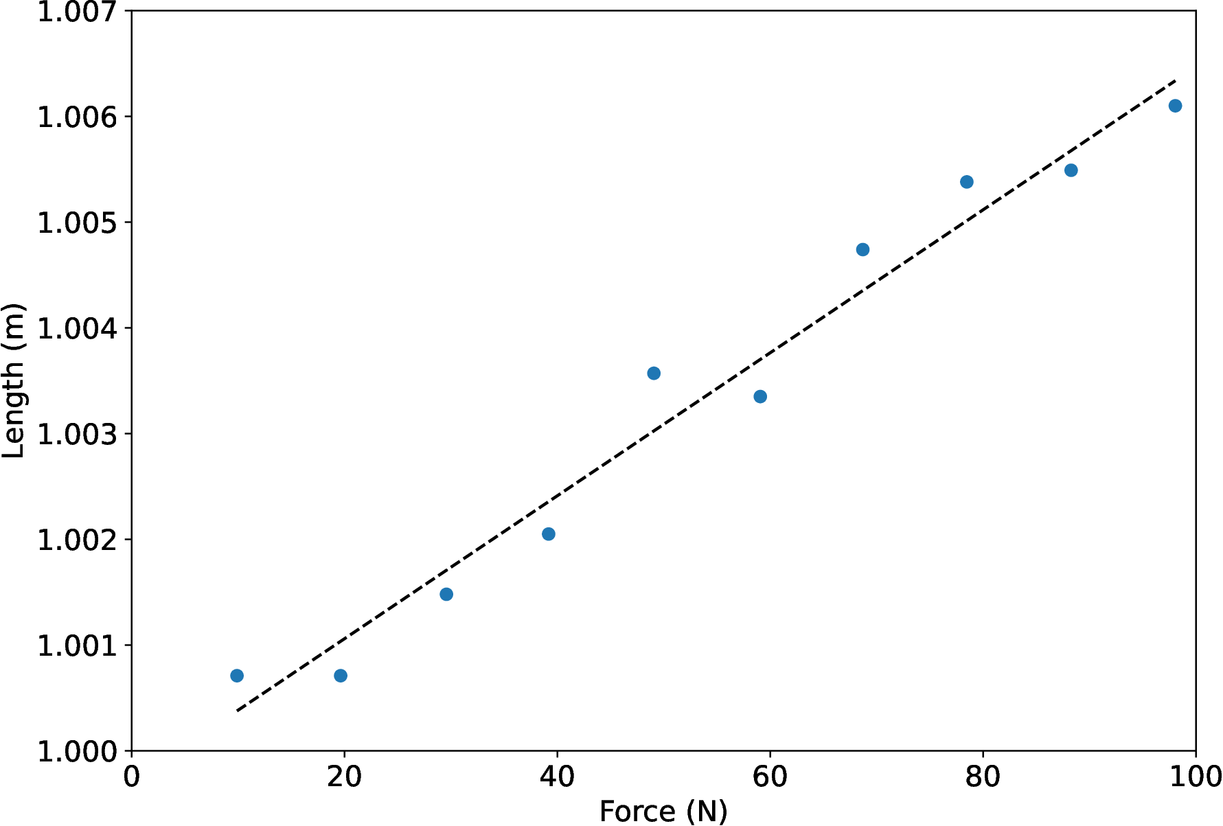
| PDF | PNG | 11.10 | Hooke's law
|
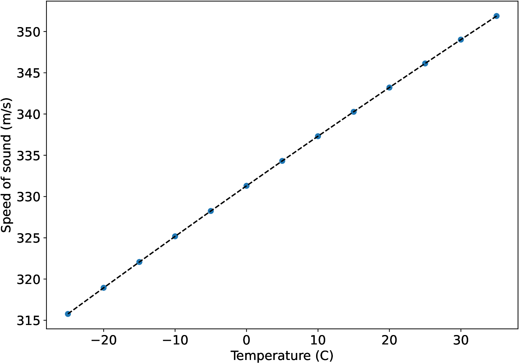
| PDF | PNG | 11.11 | Speed of sound
|
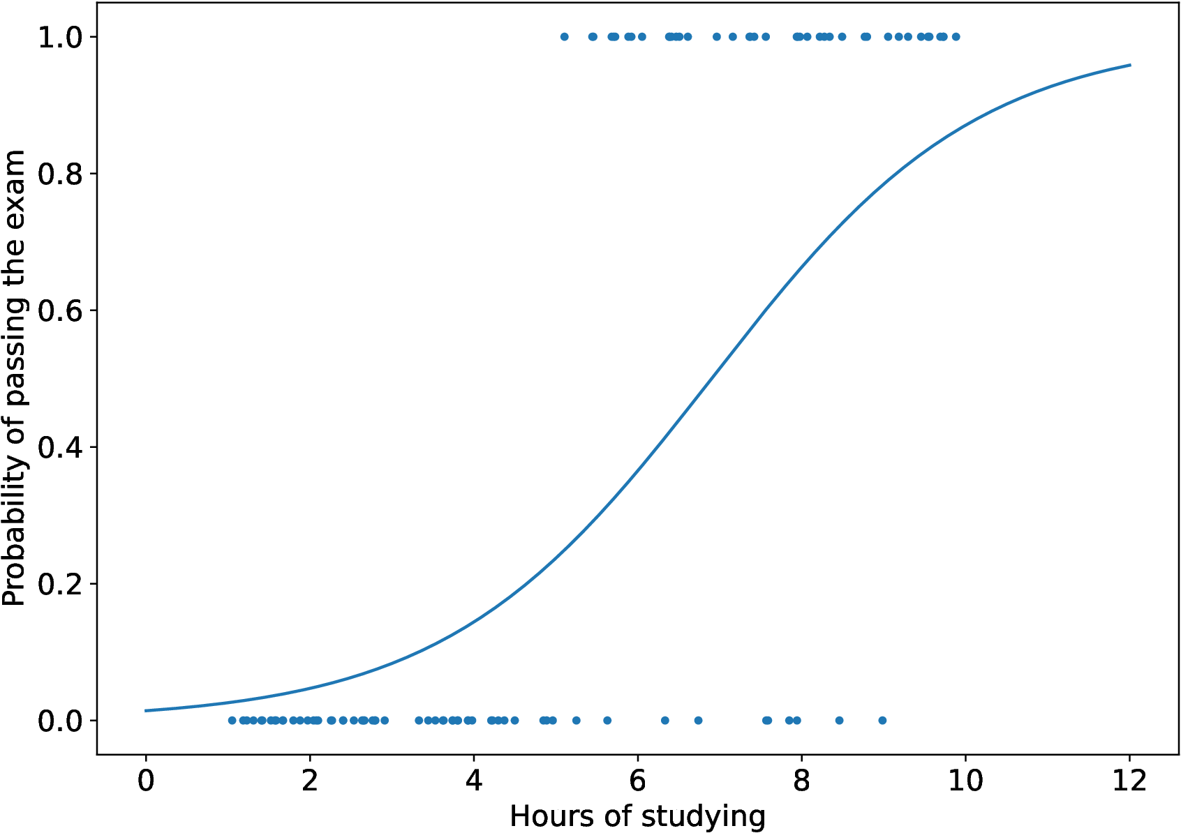
| PDF | PNG | 11.12 | Logistic regression
|
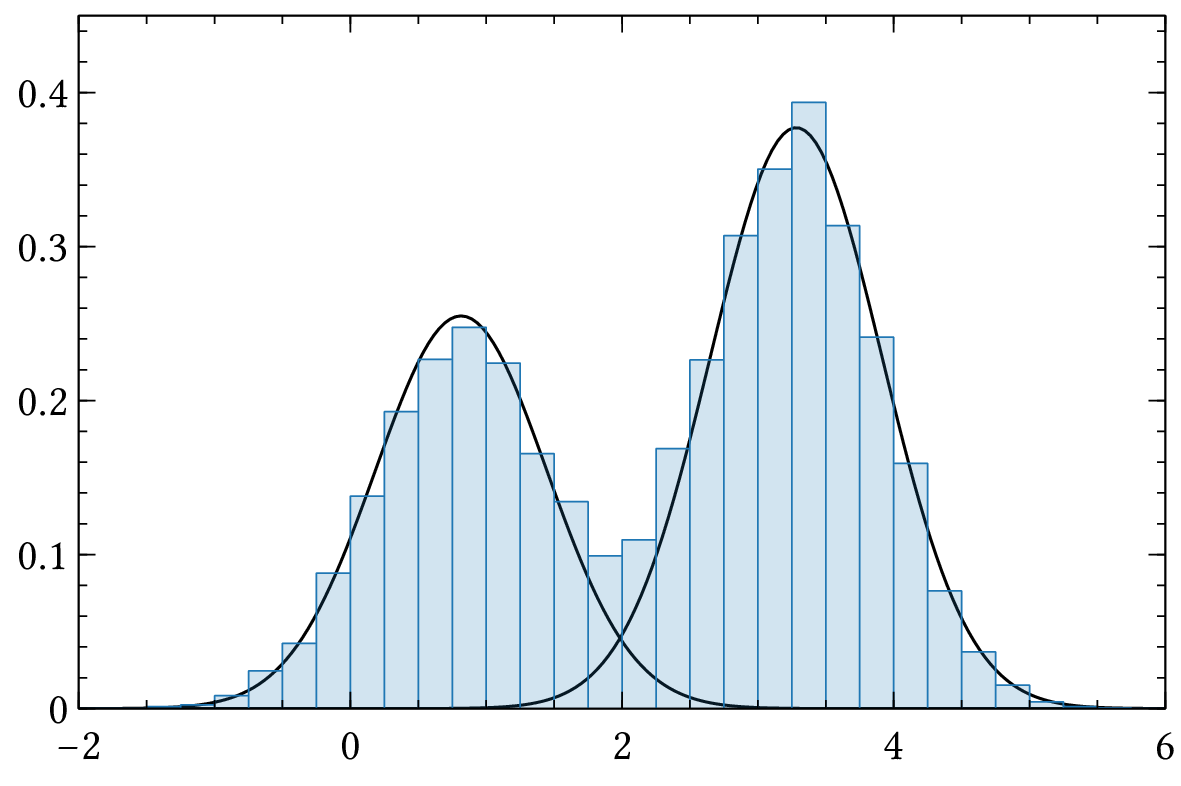
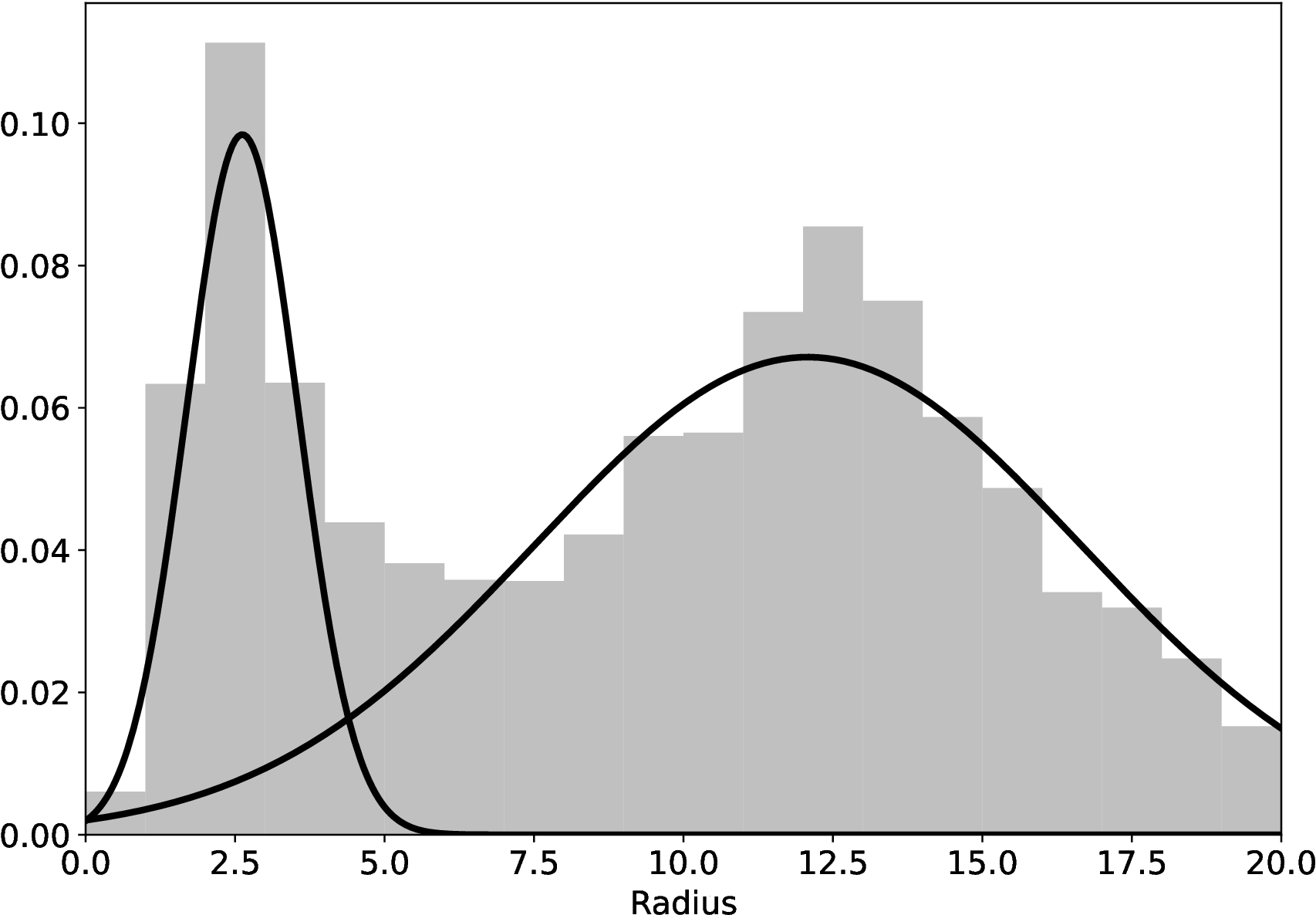
| PDF | PNG | 11.13 | Distribution with two peaks
|
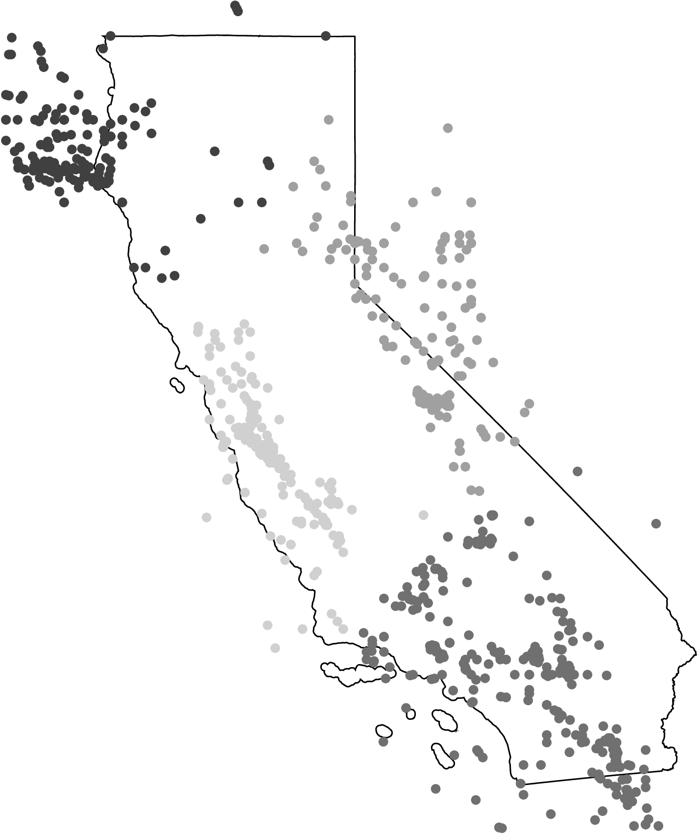
| PDF | PNG | 11.14 | Earthquakes in California
|
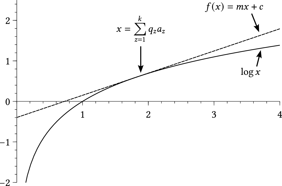
| PDF | PNG | 11.15 | Jensen's inequality
|
| PDF | PNG | 11.16 | EM algorithm for exoplanet radii
|
| PDF | PNG | 11.17 | Density estimate using EM algorithm
|
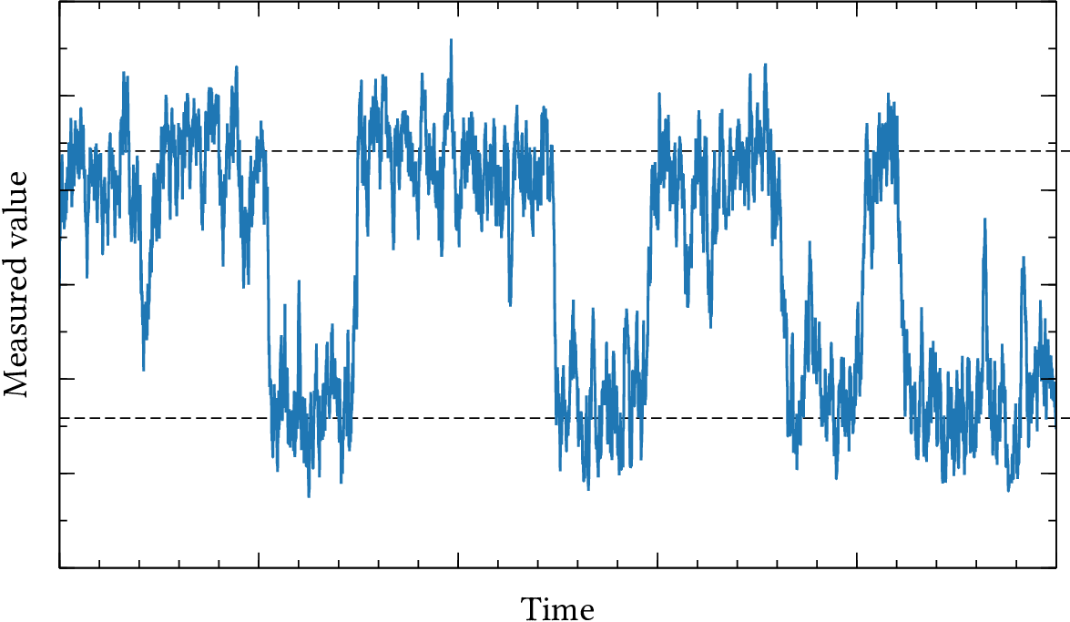
| PDF | PNG | – | Bistable physical system
|
Appendix A: Technical results
| Format | Figure | Description |
|---|
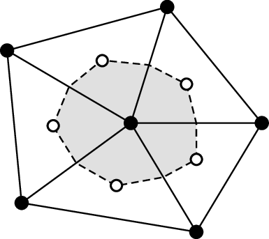
| PDF | PNG | A1a | Voronoi cell
|
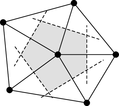
| PDF | PNG | A1b | Barycentric cell
|
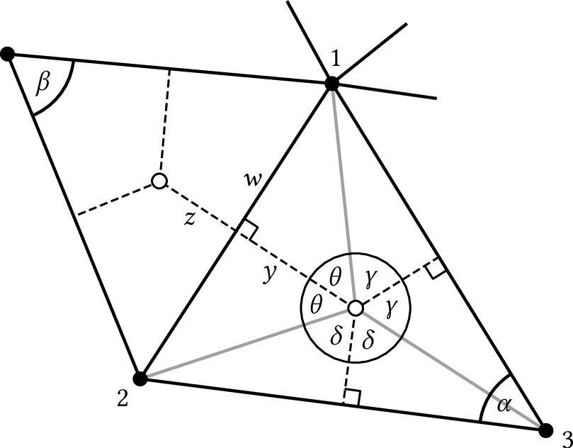
| PDF | PNG | A2 | Geometry of a triangle
|
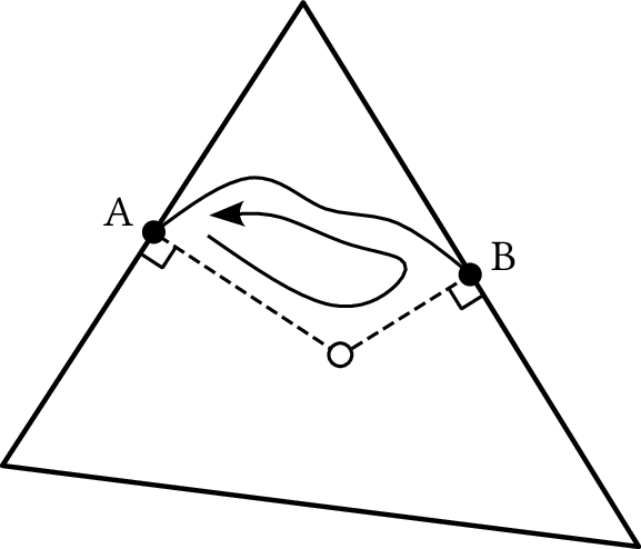
| PDF | PNG | A3 | Path independence
|