In the first stage the incumbent chooses a real value for a service type
parameter g while the opposition party chooses a challenger that has a
quality value h in the range ![]() . An increase in g
represents an increase in the concentration of benefits, while a higher value
of h represents a higher quality challenger. During the second stage
the incumbent issues a flow of proposals for a post-election district
service rate r>0, the challenger issues a flow of proposals for an
alternative service rate q>0 and the contributor issues a flow of proposals
for contributions to be made to the incumbent and challenger respectively in
amounts a>0 and b>0. The combined flow of proposals evolves continuously
according to a four-dimensional system of ordinary differential equations.
. An increase in g
represents an increase in the concentration of benefits, while a higher value
of h represents a higher quality challenger. During the second stage
the incumbent issues a flow of proposals for a post-election district
service rate r>0, the challenger issues a flow of proposals for an
alternative service rate q>0 and the contributor issues a flow of proposals
for contributions to be made to the incumbent and challenger respectively in
amounts a>0 and b>0. The combined flow of proposals evolves continuously
according to a four-dimensional system of ordinary differential equations.
The incumbent seeks to maximize both the expected gain from her service rate and the extent to which an increase in the concentration of the benefits from service helps her reelection chances. The incumbent's payoff is
![]()
where r>0 is the incumbent's service rate and p is the probability that
the incumbent wins reelection. Because the service rate r is received only
if the incumbent wins, the incumbent acts to maximize the expected value pr.
The term ![]() represents the effect an increase in the
concentration of the benefits from the service would have on the incumbent's
reelection chances. By the definition of p, below, voters are hostile to an
increase in the value of service if g >0, but respond favorably to more
service if g <0. One reason for the incumbent to care about
represents the effect an increase in the
concentration of the benefits from the service would have on the incumbent's
reelection chances. By the definition of p, below, voters are hostile to an
increase in the value of service if g >0, but respond favorably to more
service if g <0. One reason for the incumbent to care about ![]() would be if the incumbent believes that ``policy subsystems''
(Stein and Bickers 1995) or similar institutions tend to concentrate benefits
beyond the degree expressed by the incumbent's own choice of g.
would be if the incumbent believes that ``policy subsystems''
(Stein and Bickers 1995) or similar institutions tend to concentrate benefits
beyond the degree expressed by the incumbent's own choice of g.
The challenger's payoff function is similar to the incumbent's, with one modification to represent the concept of challenger quality. The challenger's payoff is
![]()
where q>0 is the challenger's service rate. Like the incumbent, the challenger seeks to maximize his expected service rate. But the degree to which the challenger is concerned about the effects of an increase in the concentration of benefits depends on the challenger's quality. The challenger is as concerned as the incumbent only if h = 1. For h<1 the challenger is less sensitive than the incumbent; if h = 0, the challenger is completely insensitive. To avoid incentive compatibility complications I assume that the party opposing the incumbent has the same payoff function as the challenger.
The contributor wishes to maximize the return it gets in service, given the amount it is committing to pay in contributions. The contributor's payoff is
![]()
where a>0 and b>0 denote the contributions made respectively to the
incumbent and the challenger. The contributor evaluates the cost of
contributions quadratically. The costs of the contributions are therefore
![]() and
and ![]() . The value of post-election service is
. The value of post-election service is ![]() if the
incumbent wins and
if the
incumbent wins and ![]() if the challenger wins.
if the challenger wins.![]() There is some service even if contributions become vanishingly
small; service is at least either
There is some service even if contributions become vanishingly
small; service is at least either ![]() or
or ![]() . But for fixed r and q
there is always more service if contributions increase. Because service is
provided only after the election, the contributor acts based on the expected
value of the potential returns, given the reelection probability p.
. But for fixed r and q
there is always more service if contributions increase. Because service is
provided only after the election, the contributor acts based on the expected
value of the potential returns, given the reelection probability p.
Such a form for K entails the idea that the contributor views campaign
contributions as investments (Snyder 1990). Given the restriction ![]() , it is easy to show that in equilibrium the contributor
gives the incumbent a contribution equal to a permanent stream of income of
one unit per period.
, it is easy to show that in equilibrium the contributor
gives the incumbent a contribution equal to a permanent stream of income of
one unit per period.![]() The specification for
K therefore implicitly represents an expected long-term relationship
between the contributor and the incumbent, whenever
The specification for
K therefore implicitly represents an expected long-term relationship
between the contributor and the incumbent, whenever ![]() . Similar results can be obtained for the challenger. The solution to
. Similar results can be obtained for the challenger. The solution to
![]() does not simplify in such an appealing way
when
does not simplify in such an appealing way
when ![]() , but the result
, but the result ![]() nonetheless gives an intuitive interpretation of the service rates r and
q. In trying to maximize r, the incumbent is trying to minimize the
interest rate at which the contributor is willing to invest in the incumbent
by making a contribution (compare Snyder 1990, 1198). For any given value of
p, a higher value of r implies a lower interest rate, and therefore a
higher ``price'' in terms of more contributions for the incumbent. The
challenger's motives are analogous.
nonetheless gives an intuitive interpretation of the service rates r and
q. In trying to maximize r, the incumbent is trying to minimize the
interest rate at which the contributor is willing to invest in the incumbent
by making a contribution (compare Snyder 1990, 1198). For any given value of
p, a higher value of r implies a lower interest rate, and therefore a
higher ``price'' in terms of more contributions for the incumbent. The
challenger's motives are analogous.
Voters treat the candidates asymmetrically in two respects. First, the incumbent enjoys a kind of recognition advantage. Voters respond to the service rate of the challenger only if the challenger succeeds in mounting a serious campaign. The classification of the challenge as serious or not occurs at the end of the game, based on the challenger's position at that time. The idea is that, through franked mail and other communications during her current term, the incumbent has already convinced the voters that she should get the benefit of the doubt in their decisions. Voters pay attention to the inherent merits of the challenger only if the media decide to cover the challenger as a worthy alternative. If this does not happen, voters take the challenger's service rate into account only when computing the value of the post-election service the challenger would provide. The media's decision is probabilistic, based on a horserace-type rule.
The second asymmetry is that the strength of voters' response to the candidates' service values depends on the level of contributions to the challenger's but not the incumbent's campaign. The idea here is that the burden is on the challenger to convince voters that they should compare the service levels the candidates are promising.
The two kinds of voter decision rules are indexed by ![]() , where
m=0 represents the situation where the challenge is not serious. Given m,
the probability that the incumbent wins is
, where
m=0 represents the situation where the challenge is not serious. Given m,
the probability that the incumbent wins is
![]()
The probability that the challenge is serious is ![]() , where
, where
![]()
with ![]() being an exogenously set constant. The challenger is likely
to be taken seriously only if he already has significant support based solely
on the comparison between his and the incumbent's service commitments. The
horserace aspect of this formulation is clearest when
being an exogenously set constant. The challenger is likely
to be taken seriously only if he already has significant support based solely
on the comparison between his and the incumbent's service commitments. The
horserace aspect of this formulation is clearest when ![]() is large, for then
is large, for then
![]() is steep near
is steep near ![]() , such that the value
, such that the value ![]() becomes in effect the
threshold below which the challenger must reduce the incumbent's support in
order to be considered a serious threat. The unconditional probability that
the incumbent wins, p, is the mixture of the serious-challenger and
not-serious-challenger alternatives:
becomes in effect the
threshold below which the challenger must reduce the incumbent's support in
order to be considered a serious threat. The unconditional probability that
the incumbent wins, p, is the mixture of the serious-challenger and
not-serious-challenger alternatives:
![]()
Voters are attracted by higher amounts of post-election service if g<0,
but repelled if g>0: ![]() and
and ![]() . The term
. The term ![]() in I can therefore give
the incumbent an incentive to reduce her service rate. The incumbent's
incentives regarding her service rate will depend on both the type of the
service and campaign contributions.
in I can therefore give
the incumbent an incentive to reduce her service rate. The incumbent's
incentives regarding her service rate will depend on both the type of the
service and campaign contributions.![]() Similar comments apply to the
challenger, so long as h > 0.
Similar comments apply to the
challenger, so long as h > 0.
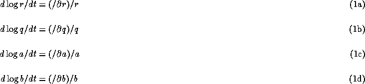
During the second stage subgame, each player uses steepest ascent with respect to its payoff function to adjust its proposal values in continuous time. To keep the proposal values positive but always with smooth dynamics, I define the differential equations in terms of the natural logarithms of the proposal variables. Using t to denote time,
There is a dynamic equilibrium when the system (1) is at a
fixed point, i.e., when ![]() . A dynamic
equilibrium is a Cournot-Nash equilibrium only if the fixed point is
a local maximum for each player, i.e., only if
. A dynamic
equilibrium is a Cournot-Nash equilibrium only if the fixed point is
a local maximum for each player, i.e., only if ![]() ,
, ![]() and the matrix
and the matrix
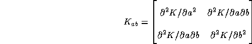
is negative definite.
The second-stage subgame that occurs for each (g, h) pair is a
realization of system (1). I assume the following about the initial
conditions for each realization. If for the (g, h) pair system
(1) has a unique Cournot-Nash equilibrium point that is
asymptotically stable (Hirsch and Smale 1974, 186), then that point is the
subgame outcome. If system (1) has multiple Cournot-Nash equilibria
for the (g, h) pair but only one equilibrium is asymptotically
stable, then the players choose the stable point.![]() Cournot-Nash equilibria that are
not asymptotically stable fixed points can be eliminated by a perfection
argument.
Cournot-Nash equilibria that are
not asymptotically stable fixed points can be eliminated by a perfection
argument.![]() If for the (g, h)
pair no stable fixed points exist, I assume that the players begin at a point
that is a Cournot-Nash equilibrium for some nearby (g, h) pair.
If for the (g, h)
pair no stable fixed points exist, I assume that the players begin at a point
that is a Cournot-Nash equilibrium for some nearby (g, h) pair.
The ideal approach to solve the game would be to integrate system (1) for a fine grid of service type and challenger quality values, and then to use the resulting payoff values to find Nash equilibria for the first-stage choices of g and h. This would be backward induction. It is computationally infeasible to integrate system (1) for so many (g, h) pairs, so I use an approximation to the ideal method. I integrate system (1) near fixed points for a large number of (g, h) pairs, the goal being to find the set of (g, h) values at which the flows of the system change in a qualitatively significant manner. Such a set is called a bifurcation set (Guckenheimer and Holmes 1986, 119). If possible, each fixed point is a stable, Cournot-Nash equilibrium. Within each region of qualitatively similar behavior relatively few integrations of system (1) are needed to determine how the payoffs to the incumbent and to the opposition party (i.e., to the challenger) vary with (g, h). For each (g, h) pair I determine payoffs from the system (1) subgame as follows. When a stable fixed point exists, payoffs are evaluated at that point. When there is a stable limit cycle but no stable fixed point, payoffs are computed by averaging around the cycle. Where stable fixed points or cycles do not exist, I use the payoffs achieved after starting near a fixed point and integrating system (1) for about two time units.