Chapter 6: Isothermal Reactor Design: Molar Flow Rates
Topics
Measures Other Than Conversion
TopUses:
A. Membrane reactors
B. Multiple reaction
Liquids: Use concentrations, i.e. CA
\( C_A = \frac{F_A}{v_0} \)
1. For the elementary liquid phase reaction \( A \rightleftharpoons B \) carried out in a CSTR, where V, vo, CAo, k, and Kc are given and the feed is pure A, the combined mole balance, rate laws, and stoichiometry are:
\( \tau = \frac{V}{v_0} = \frac{C_{A0} - C_A}{k \left[ C_A - \frac{C_B}{K_c} \right]} \)
\( \tau = \frac{C_B}{k \left[ C_A - \frac{C_B}{K_c} \right]} \)
There are two equations, two unknowns, CA and CB
Gases: Use Molar Flow Rates, I.E. Fi
\( \nu = \frac{F_T}{F_{T0}} \cdot \frac{P}{P_0} \cdot \frac{T_0}{T} \)
\( C_A = \frac{F_A}{\nu} = \frac{F_A}{v_0} \cdot \frac{F_{T0}}{F_T} \cdot \frac{P}{P_0} \cdot \frac{T_0}{T} \)
\( C_A = C_{T0} = \frac{F_A}{v_0} \cdot \left( \frac{F_A}{F_T} \right) \cdot \frac{P}{P_0} \cdot \frac{T_0}{T}, \quad C_{T0} = \frac{P_0}{R T_0} \)
2. If the above reaction, \( A \rightleftharpoons B \),carried out in the gas phase in a PFR, where V, vo,CAo,k, and Kc are given and the feed is pure A, the combined mole balance, rate laws, and stoichiometry yield, for isothermal operation (T=To) and no pressure drop (DP=0) are:
\( \frac{dF_A}{dV} = -k C_{T0} \left( \frac{F_A}{F_T} - \frac{C_{T0} \left( \frac{F_B}{F_T} \right)}{K_c} \right) \)
\( \frac{dF_B}{dV} = -k C_{T0} \left( \frac{F_A}{F_T} - \frac{C_{T0} \left( \frac{F_B}{F_T} \right)}{K_c} \right) \)
\( F_T = F_A + F_B \)
Use Polymath to plot FA and FB down the length of the reactor.
Microreactors
For isothermal microreactors, we use the same equations as a PFR as long as the flow is not laminar. If the flow is laminar, we must use the techniques discussed in chapter 13. See example 4.8 of the text.
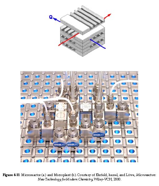
Membrane Reactors
TopMembrane reactors can be used to achieve conversions greater than the original equilibrium value. These higher conversions are the result of Le Chatelier's Principle; you can remove one of the reaction products and drive the reaction to the right. To accomplish this, a membrane that is permeable to that reaction product, but is impermeable to all other species, is placed around the reacting mixture.
Example: The following reaction is to be carried out isothermally in a membrane reactor with no pressure drop. The membrane is permeable to Product C, but it is impermeable to all other species.
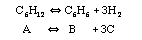
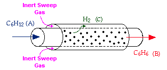
For membrane reactors, we cannot use conversion. We have to work in terms of the molar flow rates FA, FB, FC.
Polymath ProgramMole Balances
\( \frac{dF_A}{dW} = r'_A \)
\( \frac{dF_B}{dW} = r'_B = -r'_A \)
\( \frac{dF_C}{dW} = r'_C - k_c C_C = -3r'_A - k_c C_C \)
Rate Laws
\( -r'_A = k_A \left[ C_A - \frac{C_B C_C^3}{K_C} \right] \)
\( r_B = -r_A \)
\( r_C = -3r_A \)
Stoichiometry
Isothermal, no pressure drop
\( C_{T0} = \frac{P_0}{R T_0} \)
\( C_A = C_{T0} \frac{F_A}{F_T} \)
\( C_B = C_{T0} \frac{F_B}{F_T} \)
\( C_C = C_{T0} \frac{F_C}{F_T} \)
\( F_T = F_A + F_B + F_C \)
Combine
Polymath will combine for you-- Thanks Polymath...you rock!
Parameters
\( C_{T0} = \frac{0.2 \, \text{mol}}{\text{dm}^3}, \quad F_{A0} = \frac{10 \, \text{mol}}{\text{s}} \)
\( k_a = \frac{10 \, \text{dm}^3}{\text{kg cat} \cdot \text{s}}, \quad k_c = \frac{0.5 \, \text{dm}^3}{\text{kg cat} \cdot \text{s}}, \quad K_c = \frac{200 \, \text{mol}^2}{\text{dm}^6} \)
Solve
Polymath
Below are links to example problems dealing with membrane reactors. You could also use these problems as self tests.
Semibatch Reactors
TopSemibatch reactors can be very effective in maximizing selectivity in liquid phase reactions.
The reactant that starts in the reactor is always the limiting reactant.
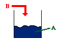
Three Forms of the Mole Balance Applied to Semibatch Reactors:
| For constant molar feed: |
\( \frac{dm}{dt} = \dot{m} \) |
|
|---|---|---|
| For constant density: |
\( m = \rho V \quad \text{and} \quad \dot{m} = \rho v_0 \) \( \frac{dV}{dt} = v_0 \) \( V = V_0 + v_0 t \) |
Use the algorithm to solve the remainder of the problem.
Example: Elementary Irreversible Reaction
Consider the following irreversible elementary reaction:
\( A + B \rightarrow C + D \)
\( -r_A = k C_A C_B \)
The combined mole balance, rate law, and stoichiometry may be written in terms of number of moles, conversion, and/or concentration:
| Conversion | Concentration | Number of Moles |
|---|---|---|
|
\[ \frac{dX}{dt} = \frac{k(1 - X)(N_{B_i} + F_{B_0}t - N_{A_0}X)}{V_0 + v_0t} \] |
\[ \frac{dC_A}{dt} = r_A - C_A \frac{v_0}{V} \] \[ \frac{dC_B}{dt} = r_A + \left(C_{B_0} - C_B\right)\frac{v_0}{V} \] |
\[ \frac{dN_A}{dt} = r_A V \] \[ \frac{dN_B}{dt} = F_{B_0} + r_B V \] |
Polymath Equations:
| Conversion | Concentration | Moles |
|---|---|---|
|
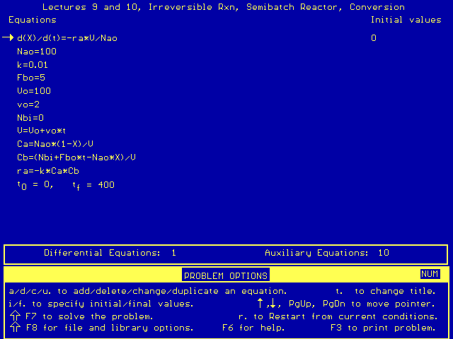
\[ \frac{dX}{dt} = -r_A \frac{V}{N_{A_0}} \] \[ r_A = -k C_A C_B \] \[ C_A = \frac{N_{A_0}(1 - X)}{V} \] \[ C_B = \frac{N_{B_i} + F_{B_0}t - N_{A_0}X}{V} \] \[ V = V_0 + v_0t \] \[ V_0 = 100, \quad v_0 = 2, \quad N_{A_0} = 100 \] \[ k = 0.1, \quad N_{B_i} = 0 \] |
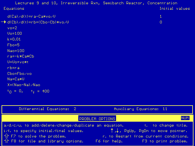
\[ \frac{dC_A}{dt} = r_A - \frac{C_A v_0}{V} \] \[ \frac{dC_B}{dt} = r_B + \frac{(C_{B_0} - C_B)v_0}{V} \] \[ r_B = r_A = -k C_A C_B \] \[ V = V_0 + v_0t \] \[ V_0 = 100, \quad v_0 = 2, \quad F_{B_0} = 5 \] \[ C_{B_0} = \frac{F_{B_0}}{v_0} \] |
\[ \frac{dN_A}{dt} = r_A V \] \[ \frac{dN_B}{dt} = r_B V + F_{B_0} \] \[ C_A = \frac{N_A}{V}, \quad C_B = \frac{N_B}{V} \] \[ X = \frac{N_{A_0} - N_A}{N_{A_0}} \] \[ k = 0.01, \quad C_A = \frac{N_A}{V} \] \[ C_B = \frac{N_B}{V} \] |
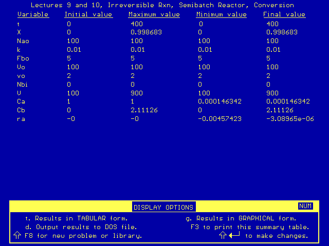
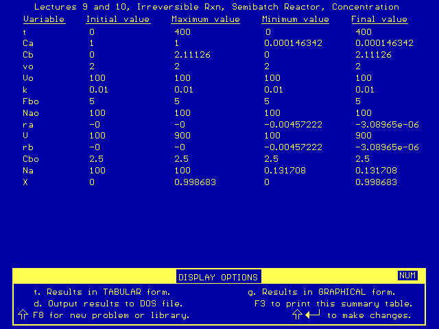
Polymath Screenshots:
| Conversion | Concentration |
|---|---|
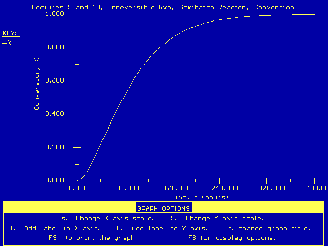
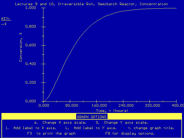
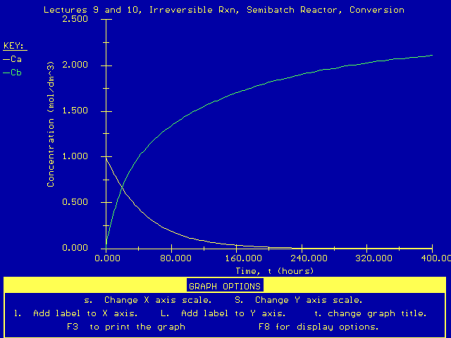
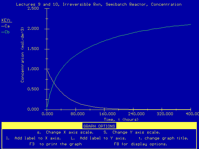
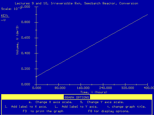
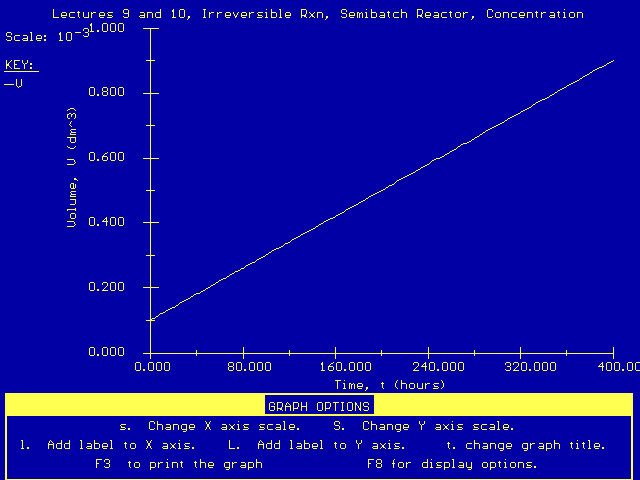
Equilibrium Conversion in Semibatch Reactors with Reversible Reactions
Consider the following reversible reaction:
\( A + B \rightleftharpoons C + D \)
Everything is the same as for the irreversible case, except for the rate law:
\( -r_A = k_A \left[ C_A C_B - \frac{C_C C_D}{K_C} \right] \)
\( C_A = \frac{N_{A0}(1 - X)}{V} \)
\( C_B = \frac{F_{B0} t - N_{A0} X}{V} \)
\( C_C = C_D = \frac{N_{A0} X}{V} \)
At equilibrium, -rA=0, then
\( -r_A = k_A \left[ C_A C_B - \frac{C_C C_D}{K_C} \right] \)
See Also:
Polymath Book Problems
A. Chapter 6 PBR ODE Solver Algorithm
PFR with Pressure Drop
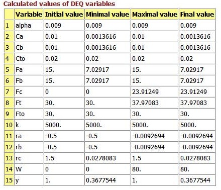
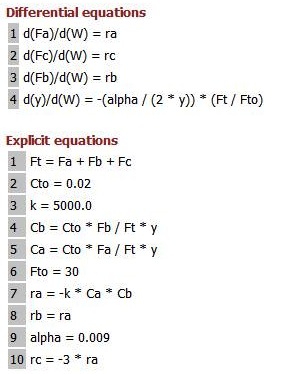
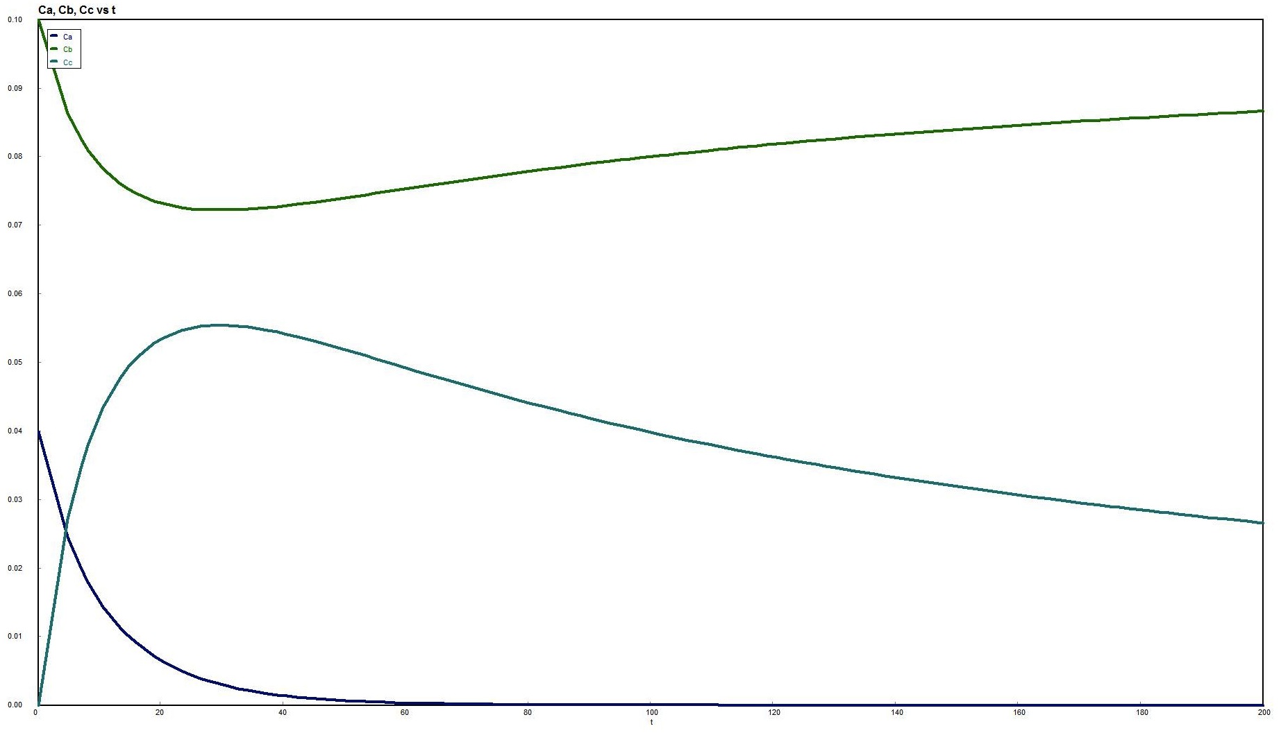
The following is an example problem from the book. It is located on page 235 in Chapter 6. This is a problem done in polymath and the .pol file has been included for reference. The report and accompanying graphs generated in Polymath are also shown.
Note that Differential equations 4 is changed to : $ d(p)/d(W) = -(\textrm{alpha} / (2 * p)) * (Ft / Ft0) $
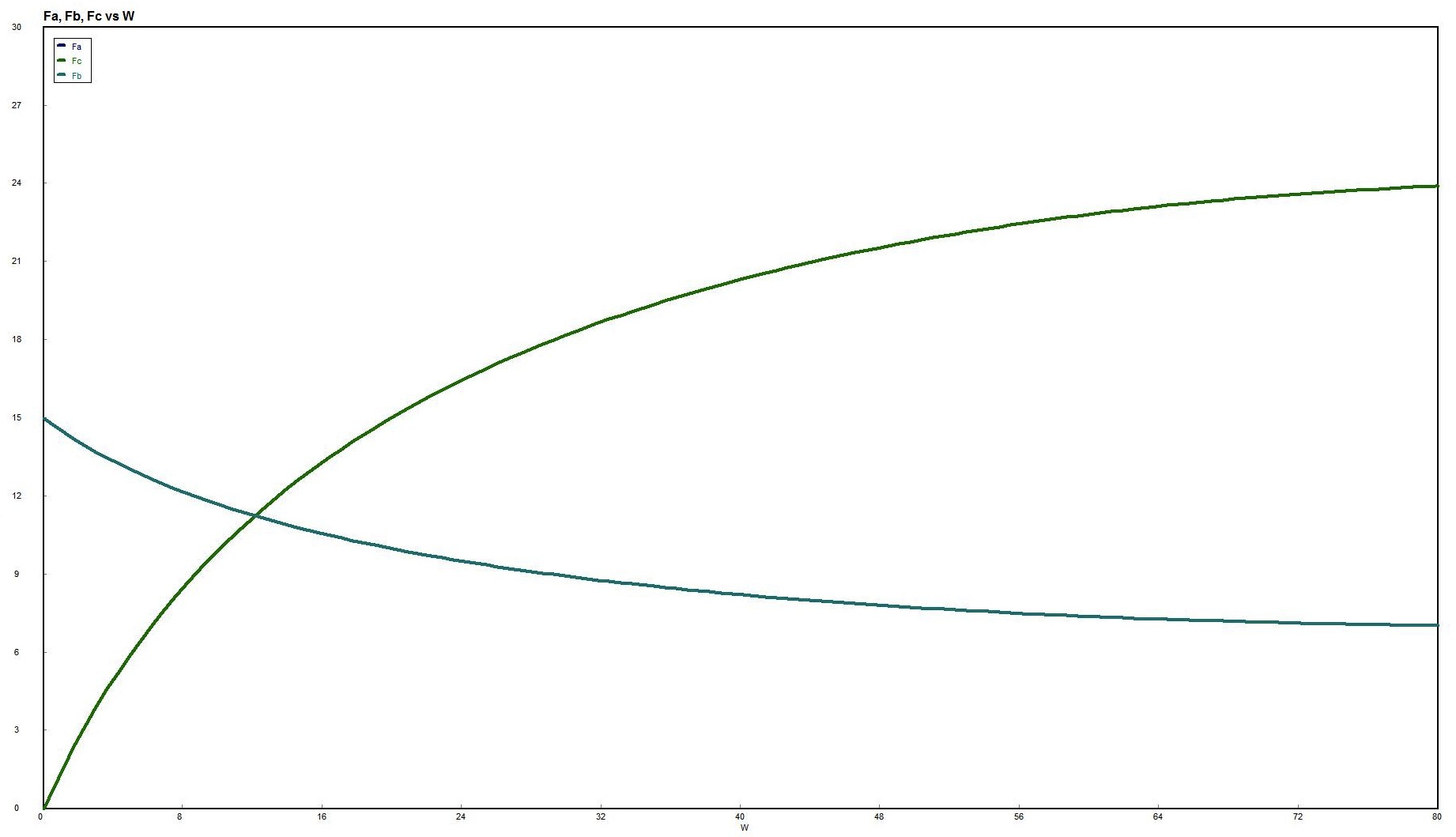
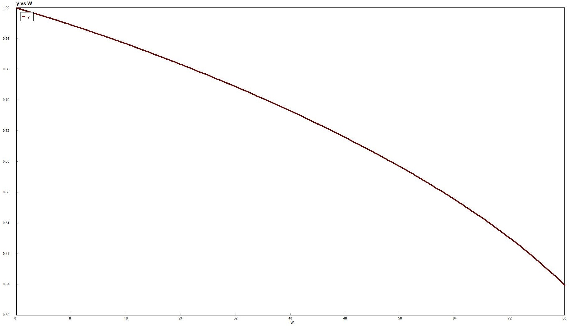
B. Chapter 6 Semibatch ODE Solver Algorithm
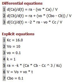
This is the second polymath problem from this chapter, shown on page 235 as well. The polymath file is included again, along with similar images.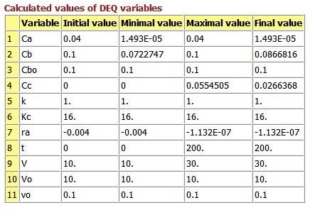
* All chapter references are for the 1st Edition of the text Essentials of Chemical Reaction Engineering .