Chapter 16: Distributions of Residence Times for Chemical Reactors
Learning Resources
Solved Problem - Example CD13-1: RTD Calculations for a Series Reaction
| Consider the reaction | |
|
|
|
|
occurring in two different reactors with the same mean residence time tm=1.26 min, but with the following residence-time distributions which are quite different: (a) Calculate the conversion predicted by an ideal |
|
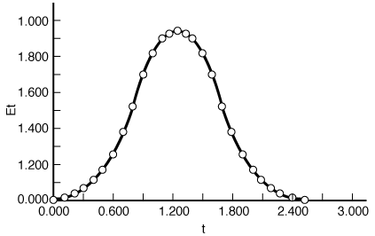
Figure CDE13-1.1 |
|
|
|
|
(c) For the multiple reaction sequence given above, determine the product distribution in each reactor for 1. The segregation model. 2. The maximum mixedness model. |
|
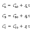
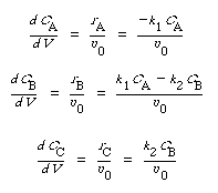
SolutionPFRCombining the mole balance and rate laws for a PFR reactor, we have |
|
|
|
(CDE13-1.1) (CDE13-1.2) (CDE13-1.3) |
|
The initial conditions are V = 0, CA = 1, CB = CC = 0. In order to compare the performance of the different models and different RTDs, the mean residence time, |
|
Table CDE13-1.1.
Polymath Program for Reactions in a Series in a PFR

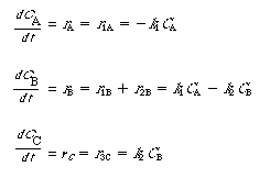
CSTR The mole balances on A, B, and C for a CSTR are |
|
|
|
(CDE13-1.4) (CDE13-1.5) (CDE13-1.6) |
|
The equations can be solved with a nonlinear equation solver. Again, |
|
|
The POLYMATH program for the CSTR model is shown in Table CDE13-1.2.The solution is CA = 0.443, CB = 0.247, CC = 0.311, X = 55.7% |
|
Table CDE13-1.2.
Polymath Program for Reactions in a Series In a CSTR
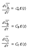
Segregation Model Combining the mole balance and rate laws for a constant-volume batch reactor, we have: For the globules |
|
|
|
(CDE13-1.7) (CDE13-1.8) (CDE13-1.9) |
| For the exit concentrations | |
|
|
(CDE13-1.10) (CDE13-1.11) (CDE13-1.12) |
|
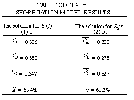
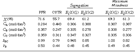
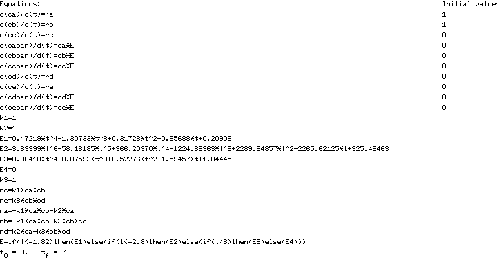
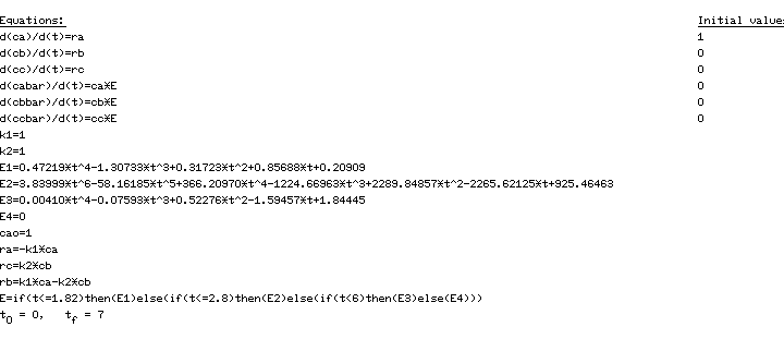
The initial conditions are t = 0, CA = 1, CB = CC = 0 The POLYMATH program used to solve these equations is shown in Table CDE13-1.3 forE1(t) (1) and in Table CDE13-1.4 for E2(t) (2).The results are listed in Table CDE13-1.5. |
|
Table CDE13-1.3. Table CDE13-1.4.
POLYMATH Program for Segregation Model with Asymmetric RTD

POLYMATH Program for Segregation Model with Bimodal Distribution
|
|
|
|
|
|
|
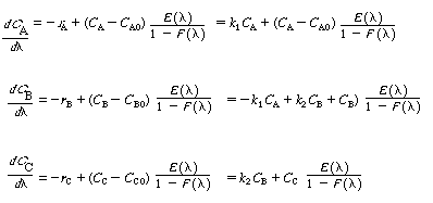
Maximum Mixedness Model The equations describing the variations in concentrations with position (life expectancy) are |
|
|
|
(CDE13-1.13) (CDE13-1.14) (CDE13-1.15) |
|
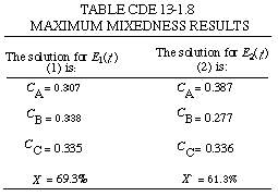
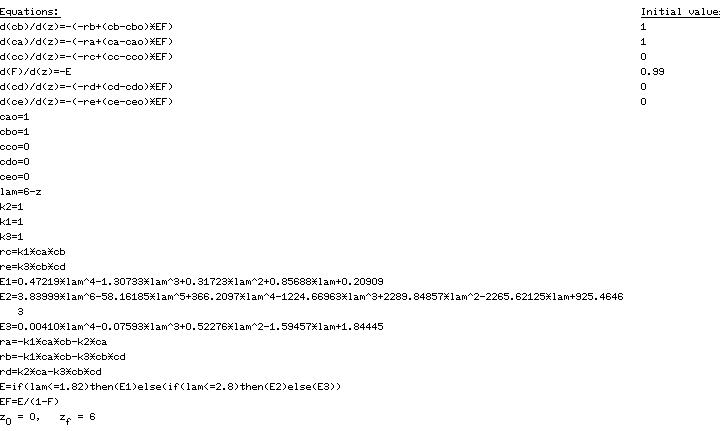
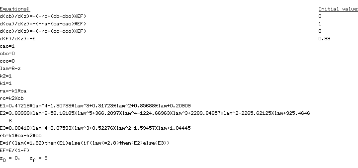
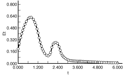
The POLYMATH program is shown in Table CDE13-1.6 for E1(t) (1)and in Table CDE13-1.7 for (2). The results are listed in Table CDE13-1.8. |
|
Table CDE13-1.6.
POLYMATH Program for Maximum Mixedness Model with Asymmetric RTD
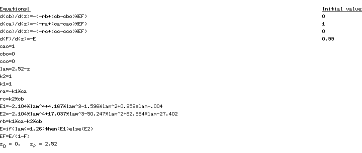
Table CDE13-1.7.
POLYMATH Program for Maximum Mixedness Model with Bimodal Distribution
|
|
|
|
Summary: Example CD13-1 |
|
|
|
|
Additional Tables for Example 13-9 Table CDE13-9.5.POLYMATH Program for Segregation Model with Bimodal Distribution (Multiple Reactions)
|
|

 , was set equal to 1.26 min.