Chapter 18: Models for Nonideal Reactors

Professional Reference Shelf

R18.2: Real Reactor Modeled as an Ideal CSTR with an Exchange Volume



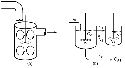
	In this particular model there is a highly agitated region in the vicinity of the impeller; outside this region, there is a region with less agitation (Figure R14.2-1). There is considerable material transfer between the two regions. Both inlet and outlet flow channels connect to the highly agitated region. We shall model the highly agitated region as one CSTR, the quieter region as another CSTR, with material transfer between the two. The material balances describing the steady-state behavior of the two reactors are

	Figure R14.2-1 (a) Real reaction systems; (b) model reaction system

Mole balances		(R14.2-1) (R14.2-2)
	The two parameters in this model are the exchange flow rate and the volume of the highly agitated region, V₁. Note that the measured volume V is just the sum of V₁ and V₂.

	These two simultaneous algebraic equations can readily be solved for most rate laws. We shall first consider the case of a first-order reaction:

		(R14.2-3)

	Let represent that fraction of the total flow that is exchanged between reactors 1 and 2:

		(R14.2-4)

	and let represent that fraction of the total volume V occupied by the highly
	agitated region:
Two parameters: and		(R14.2-5)

	Then

		(R14.2-6)

	The space-time is



	With these specifications the balance on reactor 2 becomes

		(R14.2-7)
	Solving for C _A2 gives us

		(R14.2-8)

	Substituting this value for C _A2 into the mole balance on reactor 1, Equation (R14.1-1) yields

		(R14.2-9)
	Solving for C _A1 we have

		(R14.2-10)

	In terms of conversion,
Conversion for the two-CSTR model		(R14.2-11)
	For large values of the product ,

		(R14.2-12)

	we observe that the exit concentration is a function of the relative sizes of the reactor volumes but not of the fluid exchanged between the two volumes. This statement will also be true for the case where.. For small values of the product ,

		(R14.2-13)

Limiting situations	which shows the consistency of our equation. If is very small, we should expect no significant amount of reaction. Let's examine the case where the Damköhler number,, has an intermediate value, say = 1; then



	We shall soon show how the two parameters and may be determined from tracer tests.

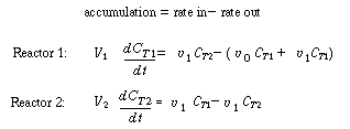
	Determination of the Parameters and . In more complex models, unfortunately, the determination of the parameters in the model is not straightforward, and they usually must be calculated by nonlinear regression using the predicted tracer response curve directly. Exceptions do exist to this general rule, though: Consider, for example, the two-CSTRs-with-interchange model described earlier (shown in Figure R14.2-2 in simplified form). A mole balance on a tracer pulse injected at t = 0 for each of the tanks is

Unsteady-state balance of inert tracer

Model system	Figure R14.2-2 Model system: two CSTRs with interchange

	C _T1 and C _T2 are the tracer concentrations in reactors 1 and 2, respectively, with C _T10 =N _T 0 /V ₁ and C _T20 = 0. As before,

		(R14.2-4) (R14.2-5)

	Substituting, we arrive at two coupled differential equations describing the unsteady behavior of the tracer that must be solved simultaneously.

		(R14.2-14) (R14.2-15)

	To obtain a solution, we first differentiate Equation (R14.2-14) with respect to u and then multiply through by (1 - ) to get
		(R14.2-16)

	Substituting Equation (R14.2-15) for the bracketed term on the right-hand side gives us

		(R14.2-17)
	The term C _T2 in Equation (R14.2-17) is eliminated by solving Equation (R14.2-14) for

Solution technique commonly encountered in reactor modeling		(R14.2-18)
	Combining Equations (R14.2-17) and (R14.2-18) and rearranging, we get
		(R14.2-19)
	which is of the form



	the solution to which is



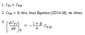
	For the problem at hand, the initial conditions at = 0 are:



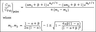
	The corresponding solution for the tracer outlet concentration is

		(R14.2-20)

Plot in C_T₁as a function of time find and	When tank 1 is rather small in comparison with tank 2 (small ), and the rates of transfer between the two reactors are small (small ), then during the first portion of the response to a pulse input the second exponential term approximates to 1. During the second portion of the response, the first exponential term approximates to zero. If the logarithm of the tracer concentration is plotted as a function of time, the response curve will approach a straight line at the two ends of the curve, and the parameters may be obtained from the slopes and intercepts of these lines. This concept has been used in physiological systems. ²