Chapter 18: Models for Nonideal Reactors

Topics

One Parameter Models
Two Parameter Models

One Parameter Models

A. Tanks-In-Series

A real reactor will be modeled as a number of equally sized tanks-in-series. Each tank behaves as an ideal CSTR. The number of tanks necessary, n (our one parameter), is determined from the E(t) curve.

For n tanks in series, E(t) is

It can be shown that

In dimensionless form

Carrying out the integration for the n tanks-in-series E(t)

For a first order reaction

For reactions other than first order and for multiple reactions the sequential equations must be solved

B. Dispersion Model

The one parameter to be determined in the dispersion model is the dispersion coefficient, D_a. The dispersion model is used most often for non-ideal tubular reactors. The dispersion coefficient can be found by a pulse tracer experiment.

After a very, very narrow pulse of tracer is injected, molecular diffusion (and eddy diffusion in turbulent flow) cause to pulse to widen as the tracer molecules diffuse randomly in all directions. The convective transport equation is:

Finding the Dispersion Coefficient

1) For laminar flow Taylor-Aris Dispersion, the molecules diffuse across radial

streamlines as well as axially to disperse the fluid.

2) To find D_a for pipes in turbulent flow see Figure 14-6

3) To find D_a for packed bed reactors see Figure 14-7

Using the RTD to find the Dispersion Coefficient.

Results of the tracer test can be used to determine Pe_r from E(t). We need to consider two sets of boundary conditions:

1. Closed-Closed Vessels

2. Open-Open Vessels

For a Closed-Closed Vessel

We note there is a discontinuity at the entering boundary in the tracer concentration.

Due to the discontinuity at boundary due to forward diffusion, C_t(O^-)=C_t0>C_t(O⁺)

However, at the end of the reactor, C_t(L^-)=C_t(L⁺)

Returning to the unsteady tracer balance

(1)

Let λ = z/L, and

Then in dimensionless form

For the closed-closed boundary condition the solution to the tracer balance at the exit (λ = 1) , at any time Θ, i.e., Ψ(1,Θ) gives

where

(2)

From page 530 of Froment and Bischoff Chemical Reactor Analysis, 2 nd Edition, John Wiley & Sons, 1966.
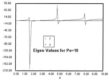
Eigen Values α_i are found from the equation

For Pe = 10
           α₁=1.5
           α₂=2.4
           α₃=4.8
           α₄=5.1
           α₅=7.9
           α₆=8.1

0 ≤ λ ≤ 1

(3)

Integrating Equation (3) using Equation (2) gives

(3)

We see from the equation for E(theta) that the exponential term dies out as the values of alpha i become large.

then t_m and Pe_r is found from the relationship:

Use RTD data to calculate t_m, ², and then P_er (i.e. D_a) and then use D_a in calculating conversion.

For the solution to with the above boundary conditions we find

For an Open-Open Vessel

Dispersion occurs upstream, downstream and within the reactor.

Pe_r>100, for long tubes, the solution at the exit is

Because of the dispersion the mean residence time is greater than the space time. The molecules can flow out of the reactor and then diffuse back in.

Use RTD data to calculate t_m, ², and then P_er (i.e. D_a) and then use D_a in calculating conversion. It can be shown that at steady state, the open-open boundary conditions reduce to the Dankwerts Boundary Conditions.

Dispersion with Reaction

For a First Order Reaction

Let Ψ = C_A/C_A0, λ = z/L , Pe = UL/D_a , and D_a = kτ. The dimensionless balance on the concentration of A in the reaction zone is

Danckwerts Boundary conditions

At λ = 0 then

At λ = 1, then

the solution is [See John B. Butt, Reaction Kinetics and Reactor Design, 2nd Edition, page 378, Marcel Dekker, 2000.]

where

The Polymath program used to plot Ψ versus λ is given below

Polymath Program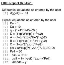

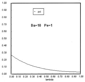
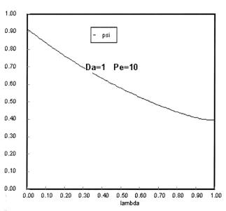
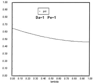
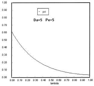
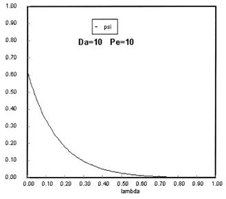
Sketches of the dimensionless concentration profiles for different values of Peclet and Damköhler numbers are shown below

Note how Ψ(0⁺) changes as Pe and D_a change.

The exit conversion is

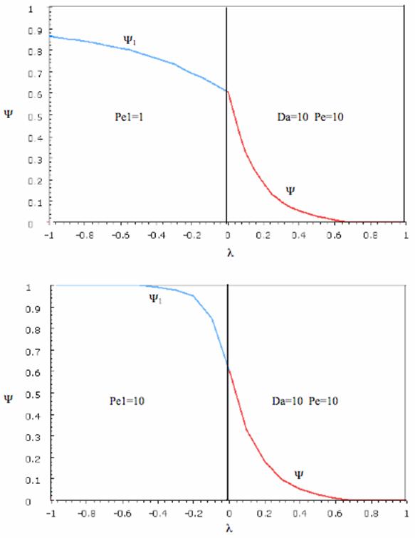
The following figures given the Polymath solutions for y versus l for different values of Pe and Da

Open Open System

Upstream of the reaction zone the balance on A in dimensionless form is

For these boundary conditions

the solution is

Rearranging

A typical profile is

The following profiles were obtained from the Polymath Program given above. Here Ψ₁ is the dimensionless concentration of A upstream of the reaction section where D_a is greater than zero and Ψ is the dimensionless concentration of A in the reaction section.

Use RTD data to calculate t_m, ², and then Pe_r (i.e. D_a) and then use D_a in calculating conversion.

Two Parameter Models

top

The goal is to model the real reactor with combinations of ideal reactors.

CSTR with Bypass and Dead Volume

Two parameters and , the fraction of volume that is well-mixed (alpha), and the fraction of the stream that is bypassed (beta).

Reactor Balance

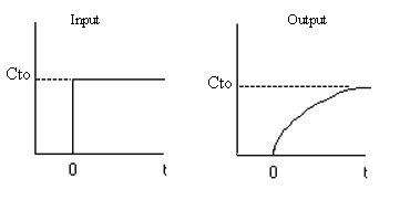
We now find the parameters a and b from a tracer experiment. We will choose a step tracer input

The balance equations are:

Finding a two parameter model

OTHER SCHEME INCLUDED

Real Reactor Model of Reactor

Two parameters, and :

Use the tracer data to find and .

Then use the mole balances and the rate law to solve for C_A1 and C_A2.

Reactor 1:
		(Eqn. A)
Rate Law:
	for a first order reaction or for a second order reaction
Reactor 2:
		(Eqn. B)
Rate Law:

Solve Equations (A) and (B) to obtain C_A1 as a function of , , k, , and C_A0.