
FEM / MATLAB
The deposition of a charged particle on a surface can be described by weak statement as follows,

Where, p represents the reduction in total free energy per unit interface area moving per unit distance,

is the magnitude of interface displacement, m is the mobility of the interface, and G is the total free energy of the system.
We used an assembly of straight line elements to approximate the charged particle deposition. The positions of the two nodes, (x1, y1,) and (x2, y2), fully specify the geometry of the element.
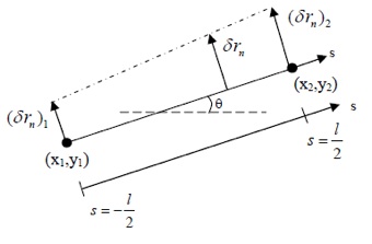
Figure: A straight line element on an interface for charged particle deposition on a surface. When the element undergoes virtual motions, the free energy varies, exerting on the two nodes several forces: the axial force, the torque, and the lateral force. [Sun et al.]


The element length is denoted by l, and the slope by theta; they relate to the nodal positions as

The virtual motion of the interface relates to the virtual motion of the nodal positions by

Where,

Here, s is the distance measured on the element starting from the mid-point of the element. Similarly, the interface velocity relates to the nodal velocities by,

The variation of total free energy associated with the virtual motion of single element is given as,

The free energy variation can be expressed in terms of virtual motions:

Here fi are the forces acting on the nodes by the element under consideration.
The left-hand side of weak statement can be expressed in terms of variations of nodal positions, velocities of nodal points, and angle theta,

Where [Hij] is a 4 x 4 symmetric matrix, also known as the viscosity matrix, is calculated from

Where N is a shape function
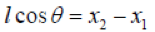
The forces on each node were calculated from free energy variation, giving
-For the case of no electric field:
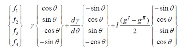
-The force column can include physical effects such as electrostatic effects:
The force and viscosity matrices are then assembled into a global matrix representing the contributions,

Then, the velocities are then solved by using Gaussian elimination, and positions are updated using Euler method.