—
Gelman Chapter 10 examples
20 Sep 2020
Chapter 10
10.1 Adding predictors to the model
We use this to match the outputs in Gelman RAOS
local gelman_output esttab,b(1) se wide mtitle("Coef.") scalars("rmse sigma") ///
    coef(_cons "Intercept" rmse "sigma") nonum noobs nostar var(15)
local gelman_output2 esttab,b(2) se wide mtitle("Coef.") scalars("rmse sigma") ///
    coef(_cons "Intercept" rmse "sigma") nonum noobs nostar var(15)
Including both predictors
page 132
import delimited https://raw.githubusercontent.com/avehtari/ROS-Examples/master/KidIQ/data/kidiq.csv,  clear
qui regress kid_score i.mom_hs c.mom_iq
`gelman_output'
(5 vars, 434 obs)
─────────────────────────────────────────
Coef.
─────────────────────────────────────────
0.mom_hs 0.0 (.)
1.mom_hs 6.0 (2.2)
mom_iq 0.6 (0.1)
Intercept 25.7 (5.9)
─────────────────────────────────────────
sigma 18.1
─────────────────────────────────────────
Standard errors in parentheses
We can graph figure 10.3 three different ways.
- first using the predicted values overlaid on scatter plots.
qui predict kid_hat
qui separate kid_hat, by(mom_hs)
twoway     (scatter kid_score mom_iq if mom_hs==0,mc(%40) mlc(%30) ms(o)) ///
        (line kid_hat0 mom_iq,sort lc(green)) ///
        (scatter kid_score mom_iq if mom_hs==1, mc(%40) mlc(%30) ms(t)) ///
        (line kid_hat1 mom_iq, sort lc(blue))  ///
        ,ytitle(Child test score) xtitle(Mother IQ score) ///
        ylab(20(40)140) xlab(80(20)140) ///
        legend(label(2 "< HS degree") label(4 "grad. HS") ///
        region(lpattern(blank)) order(2 4) pos(3) col(1)) scheme(s1color)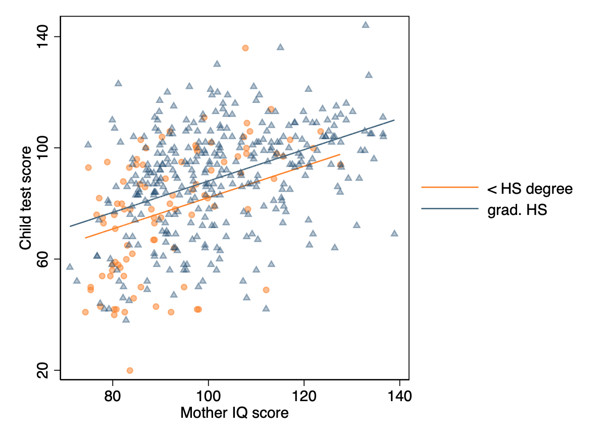
- Second by graphing the lines directly using the coefficients in a formula
twoway     (scatter kid_score mom_iq if mom_hs==0,mc(orange%50) mlc(%30) ms(o)) ///
        (function y=_b[_cons]+_b[mom_iq]*x if mom_hs==0,range(70 140) ///
            lc(orange)) ///
        (scatter kid_score mom_iq if mom_hs==1, mc(%30) mlc(%30) ms(t)) ///
        (function _b[_cons]+_b[mom_iq]*x + _b[1.mom_hs] if mom_hs==1, ///
            range(70 140) lc(edkblue))  ///
        ,ytitle(Child test score) xtitle(Mother IQ score) ///
        ylab(20(40)140) xlab(80(20)140) ///
        legend(label(2 "< HS degree") label(4 "grad. HS") ///
        region(lpattern(blank)) order(2 4) pos(3) col(1)) scheme(s1color)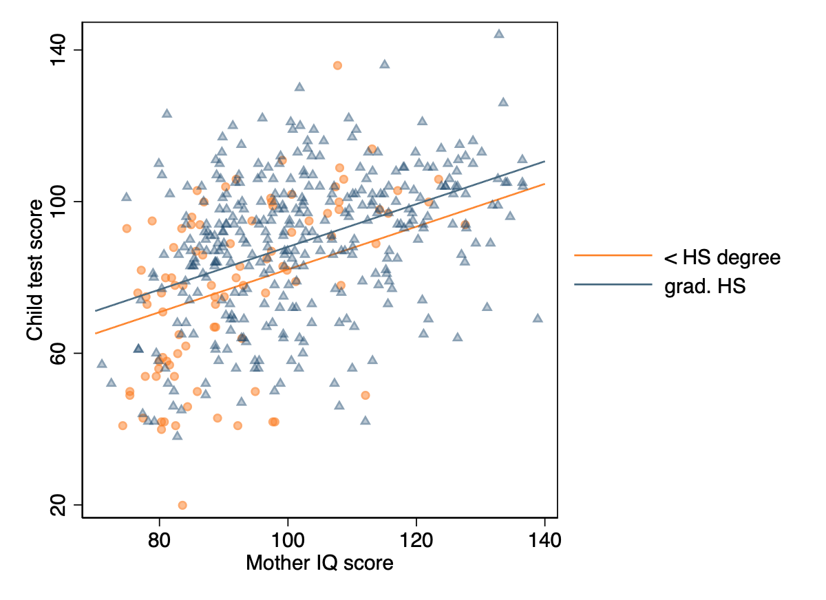
- And third by using the margins command
cap drop HS*
qui separate kid_score,by(mom_hs) gen(HS) short
qui margins mom_hs ,at(mom_iq=(60(20)140))
marginsplot, noci plot(,labels("pred. no HS" "pred. HS")) ///
    ytitle("Child test score") xtitle("Mother IQ score") title("") ///
    addplot(scatter HS0 mom_iq,ms(o)|| scatter HS1 mom_iq,ms(oh) )
Variables that uniquely identify margins: mom_iq mom_hs

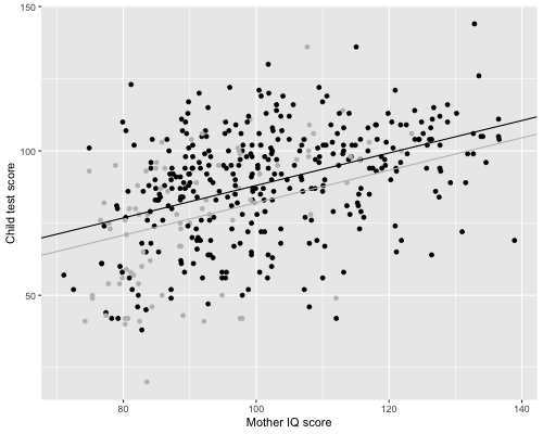
Corresponding R code and graph from 10.1
This uses approach 2 by overlaying a line plotted with the regression equation
> kidiq <- read.csv("https://raw.githubusercontent.com/avehtari/ROS-Examples/master/KidIQ/data/kidiq.csv")
> fit_3<- rstanarm::stan_glm(kid_score ~ mom_hs + mom_iq, data=kidiq, refresh=0)
> print(fit_3, detail=FALSE)
            Median MAD_SD
(Intercept) 25.8    5.7
mom_hs       6.0    2.3
mom_iq       0.6    0.1

Auxiliary parameter(s):
      Median MAD_SD
sigma 18.2    0.6
> library(ggplot2)
> png("img/fig10_3.png", width=500, height=400)
> ggplot(kidiq, aes(mom_iq, kid_score)) +
+   geom_point(aes(color = factor(mom_hs)), show.legend = FALSE) +
+   geom_abline(
+ intercept = c(coef(fit_3)[1], coef(fit_3)[1] + coef(fit_3)[2]),
+ slope = coef(fit_3)[3],
+ color = c("gray", "black")) +
+   scale_color_manual(values = c("gray", "black")) +
+   labs(x = "Mother IQ score", y = "Child test score")
> invisible(dev.off())
10.2 Interpreting regression coefficients
10.3 Interactions
* regress kid_score i.mom_hs mom_iq i.mom_hs#c.mom_iq // same as below
qui regress kid_score i.mom_hs##c.mom_iq
`gelman_output'
─────────────────────────────────────────
Coef.
─────────────────────────────────────────
0.mom_hs 0.0 (.)
1.mom_hs 51.3 (15.3)
mom_iq 1.0 (0.1)
0.mom_hs#c.mo~q 0.0 (.)
1.mom_hs#c.mo~q -0.5 (0.2)
Intercept -11.5 (13.8)
─────────────────────────────────────────
sigma 18.0
─────────────────────────────────────────
Standard errors in parentheses
cap drop kid_hat*
qui predict kid_hat
qui separate kid_hat, by(mom_hs)
twoway     (scatter kid_score mom_iq if mom_hs==0,mc(orange%50) mlc(%30) ms(o)) ///
        (line kid_hat0 mom_iq,sort lc(orange)) ///
        (scatter kid_score mom_iq if mom_hs==1, mc(%30) mlc(%30) ms(t)) ///
        (line kid_hat1 mom_iq, sort lc(edkblue))  ///
        ,ytitle(Child test score) xtitle(Mother IQ score) ///
        ylab(20(40)140) xlab(80(20)140) ///
        legend(label(2 "< HS degree") label(4 "grad. HS") ///
        region(lpattern(blank)) order(2 4) pos(3) col(1)) scheme(s1color)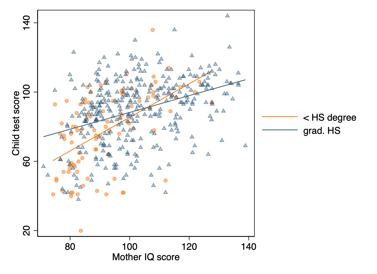
10.4 Indicator variables
import delimited  https://raw.githubusercontent.com/avehtari/ROS-Examples/master/Earnings/data/earnings.csv, clear numericcols(2)
li height weight male earn ethnicity education walk exercise smokenow tense angry age in 1/5
regress weight height
sum height,meanonly
di "Predicted weight for a 66-inch-tall person is " round(_b[_cons]+`r(mean)'*_b[height],1.1) " pounds with a sd of - difficult to get manually but you can use margins"
margins,at(height=`r(mean)')
┌─────────────────────────────────────────────────────────────────────────────────────────────────────────┐
│ height weight male earn ethnic~y educat~n walk exercise smokenow tense angry age │
├─────────────────────────────────────────────────────────────────────────────────────────────────────────┤
1. │ 74 210 1 50000 White 16 3 3 2 0 0 45 │
2. │ 66 125 0 60000 White 16 6 5 1 0 0 58 │
3. │ 64 126 0 30000 White 16 8 1 2 1 1 29 │
4. │ 65 200 0 25000 White 17 8 1 2 0 0 57 │
5. │ 63 110 0 50000 Other 16 5 6 2 0 0 91 │
└─────────────────────────────────────────────────────────────────────────────────────────────────────────┘
─────────────────────────────────────────
Coef.
─────────────────────────────────────────
height 4.9 (0.2)
Intercept -173.3 (11.9)
─────────────────────────────────────────
sigma 29.0
─────────────────────────────────────────
Standard errors in parentheses
Predicted weight for a 66-inch-tall person is 156.2
The standard error is difficult to compute manually but we can use margins to get the same thing.
. margins,at(height=`r(mean)')

Adjusted predictions                            Number of obs     =      1,789
Model VCE    : OLS

Expression   : Linear prediction, predict()
at           : height          =    66.56883

─────────────┬────────────────────────────────────────────────────────────────
             │            Delta-method
             │     Margin   Std. Err.      t    P>|t|     [95% Conf. Interval]
─────────────┼────────────────────────────────────────────────────────────────
       _cons │    156.188   .6845229   228.17   0.000     154.8455    157.5306
─────────────┴────────────────────────────────────────────────────────────────
Center variables
We are told the average height of American adults is 66 inches.
gen c_height=height-66
qui regress weight c_height
`gelman_output'
─────────────────────────────────────────
Coef.
─────────────────────────────────────────
c_height 4.9 (0.2)
Intercept 156.2 (0.7)
─────────────────────────────────────────
sigma 29.0
─────────────────────────────────────────
Standard errors in parentheses
Include binary variable in a regression
To compute the predicted weight for a 70 inch woman or a 70 inch man
. qui regress weight c_height i.male

. `gelman_output'

─────────────────────────────────────────
                       Coef.
─────────────────────────────────────────
c_height                 3.9        (0.3)
0.male                   0.0          (.)
1.male                  11.8        (2.0)
Intercept              151.7        (1.0)
─────────────────────────────────────────
sigma                   28.7
─────────────────────────────────────────
Standard errors in parentheses

. margins i.male ,at(c_height=4)

Adjusted predictions                            Number of obs     =      1,789
Model VCE    : OLS

Expression   : Linear prediction, predict()
at           : c_height        =           4

─────────────┬────────────────────────────────────────────────────────────────
             │            Delta-method
             │     Margin   Std. Err.      t    P>|t|     [95% Conf. Interval]
─────────────┼────────────────────────────────────────────────────────────────
        male │
          0  │   167.2985   1.753874    95.39   0.000     163.8586    170.7384
          1  │   179.1356   1.110306   161.34   0.000      176.958    181.3132
─────────────┴────────────────────────────────────────────────────────────────
indicator variables for multiple levels
. encode ethnicity,gen(ethn_cat)

. qui regress weight c_height i.male i.ethn_cat

. `gelman_output'

─────────────────────────────────────────
                       Coef.
─────────────────────────────────────────
c_height                 3.9        (0.3)
0.male                   0.0          (.)
1.male                  12.1        (2.0)
1.ethn_cat               0.0          (.)
2.ethn_cat              -6.2        (3.6)
3.ethn_cat             -12.3        (5.2)
4.ethn_cat              -5.2        (2.3)
Intercept              156.5        (2.3)
─────────────────────────────────────────
sigma                   28.6
─────────────────────────────────────────
Standard errors in parentheses
Change the base levels
. qui regress weight c_height i.male ib4.ethn_cat

. `gelman_output'

─────────────────────────────────────────
                       Coef.
─────────────────────────────────────────
c_height                 3.9        (0.3)
0.male                   0.0          (.)
1.male                  12.1        (2.0)
1.ethn_cat               5.2        (2.3)
2.ethn_cat              -1.0        (2.9)
3.ethn_cat              -7.1        (4.8)
4.ethn_cat               0.0          (.)
Intercept              151.3        (1.0)
─────────────────────────────────────────
sigma                   28.6
─────────────────────────────────────────
Standard errors in parentheses
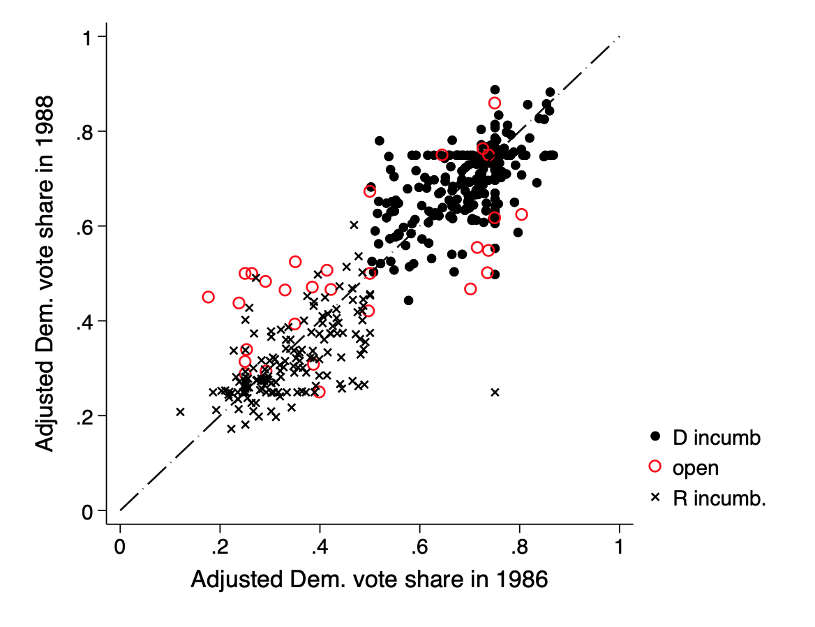
10.6 Example: Uncertainty in predicting congressional elections
qui import delimited "https://raw.githubusercontent.com/avehtari/ROS-Examples/master/Congress/data/congress.csv" ,clear
gen vote=v88
gen past_vote=v86_adj
gen inc=inc88
qui regress vote past_vote inc
`gelman_output2'
─────────────────────────────────────────
Coef.
─────────────────────────────────────────
past_vote 0.52 (0.03)
inc 0.10 (0.01)
Intercept 0.24 (0.02)
─────────────────────────────────────────
sigma 0.07
─────────────────────────────────────────
Standard errors in parentheses
. twoway (scatter vote past_vote if inc88==1,m(o)) ///
>     (scatter vote past_vote if inc88==0,mc(red))  ///
>     (scatter vote past_vote if inc88==-1,m(X)) ///
>     (function y=x , range(0 1)), ///
>     ysize(5) xsize(6.5) legend(order(1 "D incumb" 2 "open" 3 "R incumb.")) ///
>     xtitle("Adjusted Dem. vote share in 1986") ///
>     ytitle("Adjusted Dem. vote share in 1988")