—
Gelman Chapter 11.3-11.5 examples
24 Sep 2020
Use for outputs
local gelman_output esttab,b(1) se wide mtitle("Coef.") scalars("rmse sigma") ///
    coef(_cons "Intercept" rmse "sigma") nonum noobs nostar var(15)
local gelman_output2 esttab,b(2) se wide mtitle("Coef.") scalars("rmse sigma") ///
    coef(_cons "Intercept" rmse "sigma") nonum noobs nostar var(15)
Chapter 11.3-11.5
11.3 Residual plots
Residual plot adding lines for mean=0 and +/- 1 standard deviation (using the root mean squared error from the regression)
import delimited https://raw.githubusercontent.com/avehtari/ROS-Examples/master/KidIQ/data/kidiq.csv,  clear
qui regress kid_score mom_hs mom_iq
rvfplot ,yline(0) yline(-`e(rmse)' `e(rmse)', lp(dash))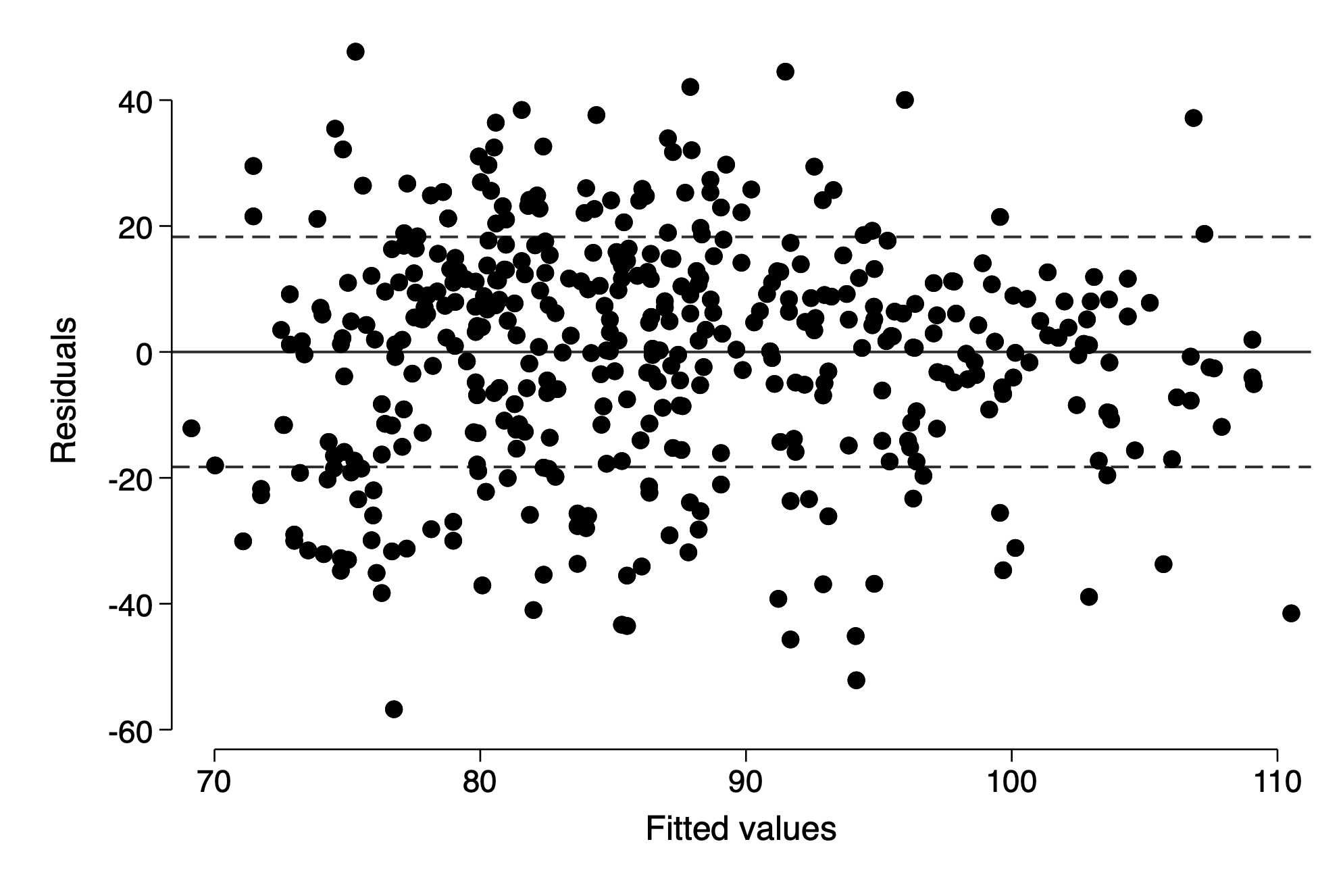
Using fake data to understand residual plots
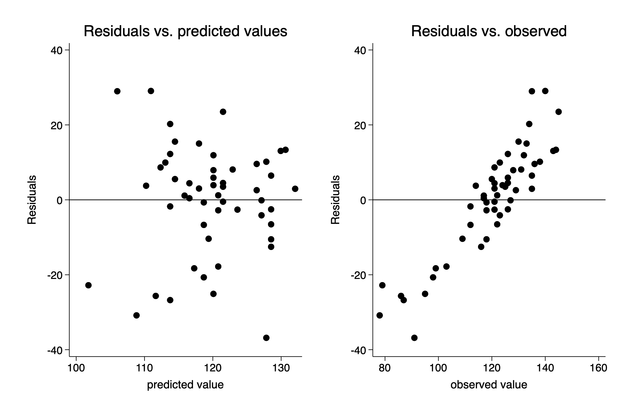
Residuals vs predicted or vs. observed?
qui import delimited  https://raw.githubusercontent.com/avehtari/ROS-Examples/master/Introclass/data/gradesW4315.dat, delim(" \t",collapse)  clear
qui regress final midterm
`gelman_output'
rvfplot ,yline(0) title(Residuals vs. predicted values)  ///
    xtitle(predicted value) name(fig11_7_stata_a,replace)
predict final_resid,resid
scatter final_resid final, yline(0) title(Residuals vs. observed) ///
    name(fig11_7_stata_b, replace) xtitle(observed value)
graph combine fig11_7_stata_a fig11_7_stata_b
(11 vars, 52 obs)
─────────────────────────────────────────
Coef.
─────────────────────────────────────────
midterm 0.7 (0.2)
Intercept 64.5 (17.0)
─────────────────────────────────────────
sigma 14.8
─────────────────────────────────────────
Standard errors in parentheses
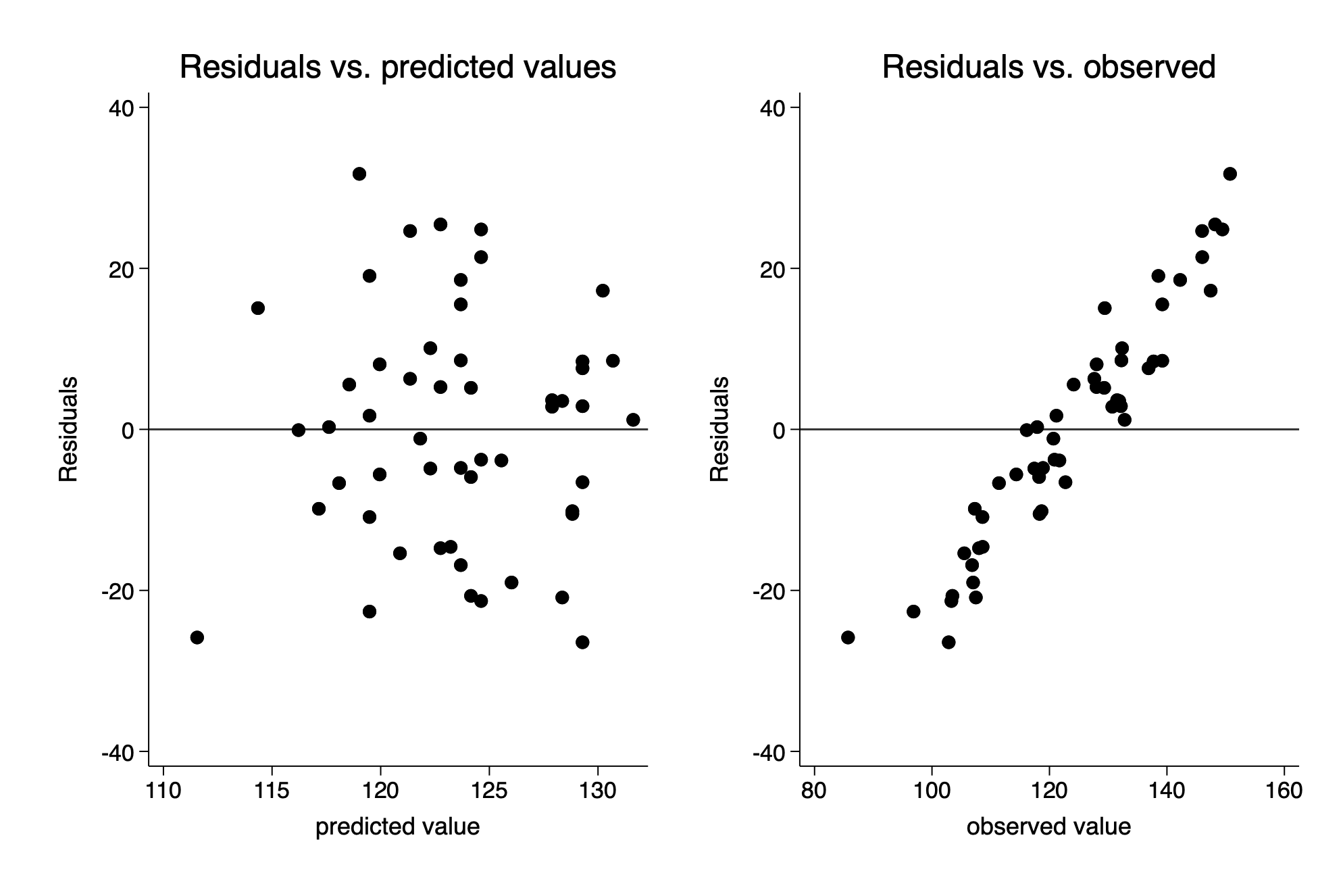
Understanding the choice using fake data
local a=64.5
local b=0.7
local sigma=14.8
gen final_fake=`a' + `b'*midterm + rnormal(0, `sigma')
qui regress final_fake midterm
`gelman_output'
rvfplot ,yline(0) title(Residuals vs. predicted values) xtitle(predicted value) ///
    name(fig11_8_stata_a,replace)
cap drop final_resid
predict final_resid,resid
scatter final_resid final_fake, yline(0) title(Residuals vs. observed) ///
    name(fig11_8_stata_b, replace) xtitle(observed value)
graph combine fig11_8_stata_a fig11_8_stata_b
─────────────────────────────────────────
Coef.
─────────────────────────────────────────
midterm 0.5 (0.2)
Intercept 86.8 (16.8)
─────────────────────────────────────────
sigma 14.6
─────────────────────────────────────────
Standard errors in parentheses
11.4 Comparing data to replications from a fitted model
Example: simulation based checking of a fitted normal distribution
The data
qui import delimited https://raw.githubusercontent.com/avehtari/ROS-Examples/master/Newcomb/data/newcomb.txt ,clear
hist y, fc(white) ysc(off) xtitle("")  discrete width(2)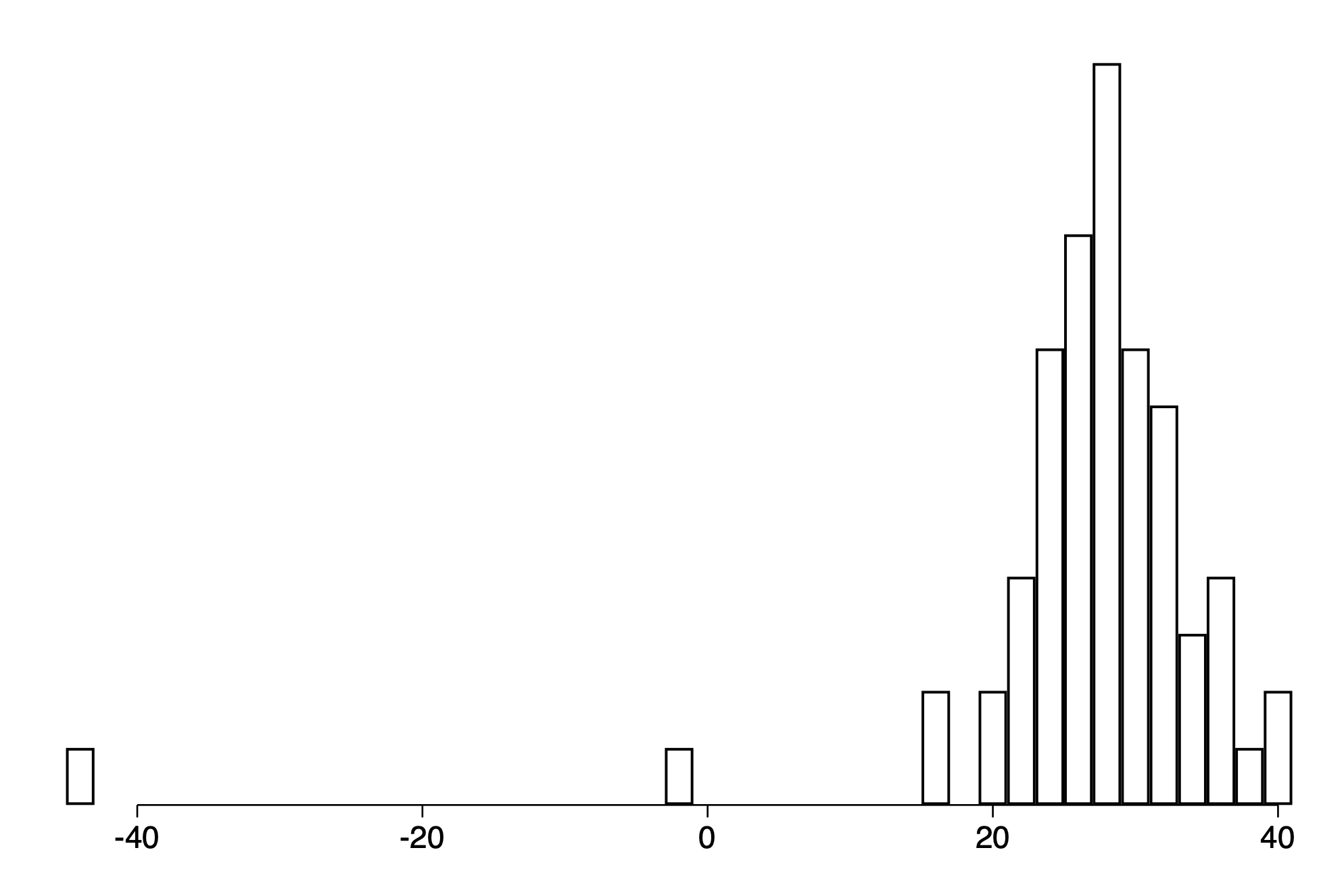
Visual comparison of actual and replicated datasets
Fitting (inappropriately) a normal distribution to the data by a simple empty regression of y. Given the assumption of normal distribution of the error term in regression, this forces any deviations around the mean to be normally distributed)
We construct replicated data differently than in Gelman. They use bayesian regression for all their examples. As the estimation is done by simulation they already have replicates of the coefficients and error term which they summarize for the model output. It is trivial then to generate a new outcome by plugging the data into the different sets of coefficients with the error term.
As we use maximum likelihood methods, we treat the coefficients as fixed and the data as random
So we combine our estimate of the coefficient with a draw from the error term to generate a new value.
qui regress y
cap drop y_r*
forval i=1/20    {
    qui gen y_r`i'=_b[_cons] + rnormal(0,`e(rmse)')
    qui hist y_r`i',name(y_r`i',replace) fc(white) ysc(off) xtitle("")
}
unab yhist: y_r*
graph combine `yhist'
qui graph export img/fig11_10_stata.png,replace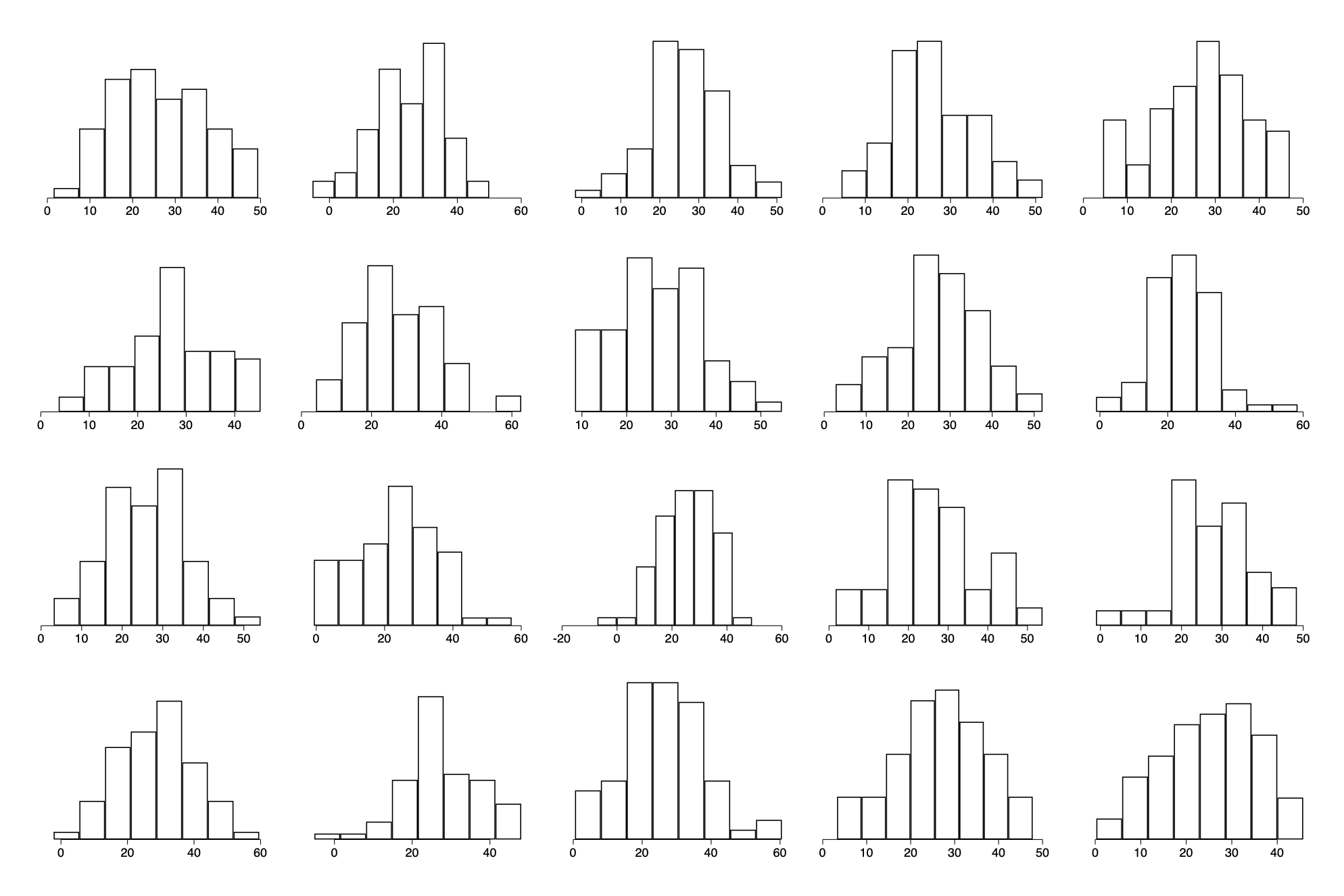
Alternate visualization on a single axis
twoway kdensity y || kdensity y_r1,lc(gs14) lpatt(solid) ||  ///
    kdensity y_r2,lc(gs14) lpatt(solid) || kdensity y_r3,lc(gs14) lpatt(solid) || ///
    kdensity y_r4,lc(gs14) lpatt(solid) || kdensity y_r5,lc(gs14) lpatt(solid) || ///
    kdensity y_r6,lc(gs14) lpatt(solid) || kdensity y_r7,lc(gs14) lpatt(solid) || ///
    kdensity y_r8,lc(gs14) lpatt(solid) || kdensity y_r9,lc(gs14) lpatt(solid) || ///
    kdensity y_r10,lc(gs14) lpatt(solid) || kdensity y_r11,lc(gs14) lpatt(solid) || ///
    kdensity y_r12,lc(gs14) lpatt(solid) || kdensity y_r13,lc(gs14) lpatt(solid) || ///
    kdensity y_r14,lc(gs14) lpatt(solid) || kdensity y_r15,lc(gs14) lpatt(solid) || ///
    kdensity y_r16,lc(gs14) lpatt(solid) || kdensity y_r17,lc(gs14) lpatt(solid) || ///
    kdensity y_r18,lc(gs14) lpatt(solid) || kdensity y_r19,lc(gs14) lpatt(solid) || ///
    kdensity y_r20,lc(gs14) lpatt(solid) , ysc(off) xtitle("") legend(off) ///
    xlab(-25(25)50) ysc(fextend) xsc(fextend)
qui graph export img/fig11_11_stata.png,replace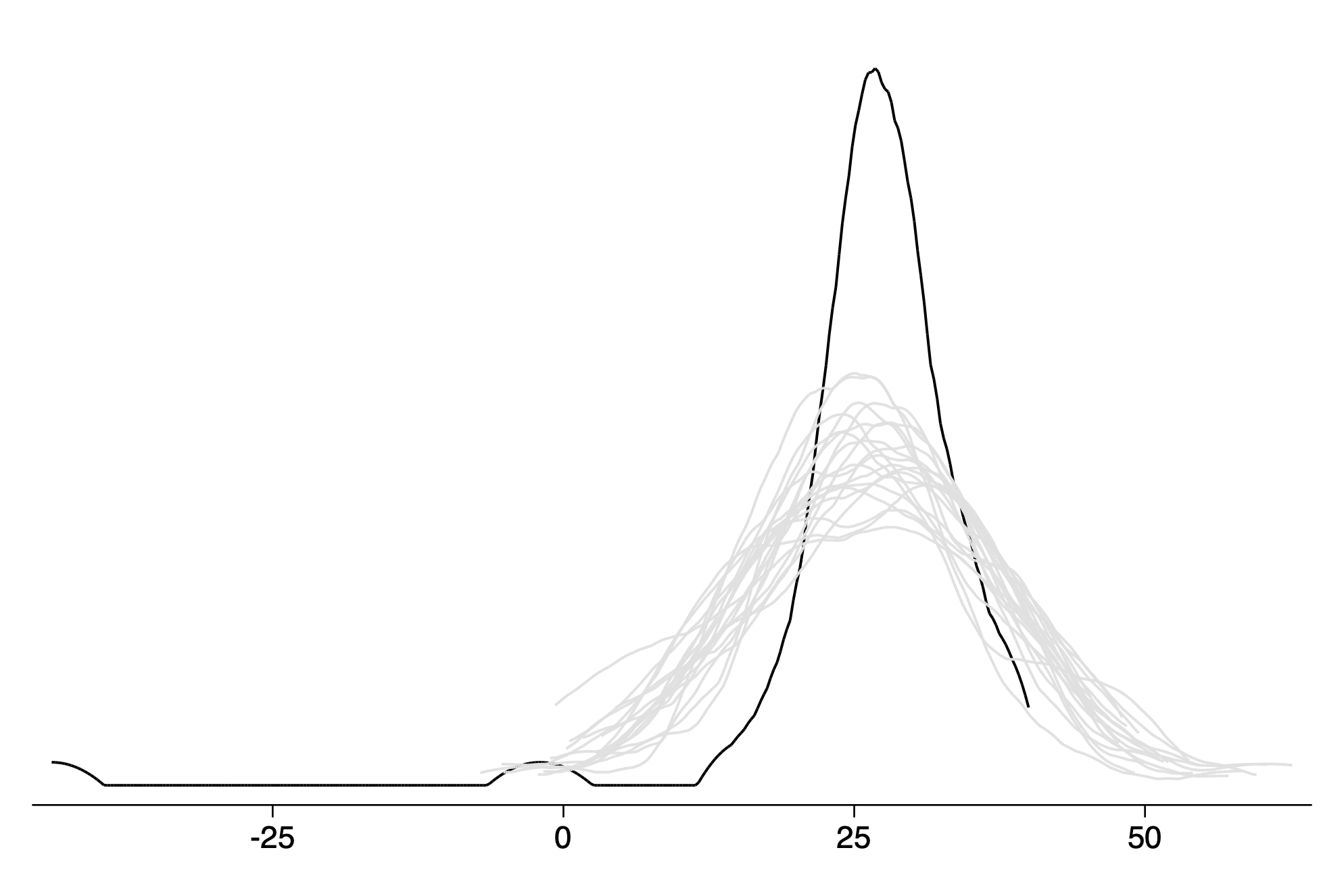
11.5 Fitting a first order autoregression to the unemployment series
import delimited  https://raw.githubusercontent.com/avehtari/ROS-Examples/master/Unemployment/data/unemp.txt, delim(" \t",collapse)  clear
gen y_lag=y[_n-1]
qui regress y y_lag
`gelman_output2'
(1 missing value generated)
─────────────────────────────────────────
Coef.
─────────────────────────────────────────
y_lag 0.77 (0.08)
Intercept 1.35 (0.46)
─────────────────────────────────────────
sigma 1.02
─────────────────────────────────────────
Standard errors in parentheses
Simulating replicated datasets
Again we generate relicate datasets as described above.
cap drop y_r*
set seed 3992
forval i=1/15    {
    qui gen y_r`i'=_b[_cons]+ ///
        _b[y_lag]*y_lag + rnormal(0,`e(rmse)')
    }
Visualizing and numerical comparisons of replicated to actual data
forval i=1/15    {
    qui line y_r`i' year,sort name(y_r`i',replace) fc(white) ///
    xlab(.) ylab(.) ytick(0(1)10) xtick(1950(10)2010)  ytitle(" ") xtitle("") ///
    subtitle("Simulation `i'")
    }
unab yhist: y_r*
graph combine `yhist'
qui graph export img/fig11_14_stata.png,replace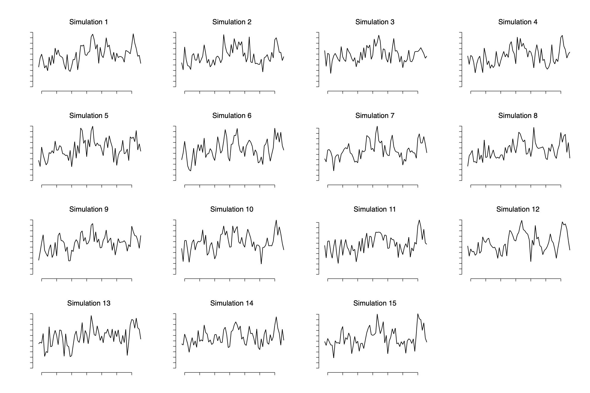
In stata it is easier to write a program to cacluate this test statistic (quantifying the relative “lack of smoothness” of the replicated data as compared to the actual data by looking at the number of switches in direction in each)
cap prog drop switch_test
prog define switch_test
    syntax varlist
    tokenize `varlist'
    local first `1'
    while "`first'"!=""    {
        tempvar y_lag y_lag2 test
        qui gen `y_lag'=`first'[_n-1]
        qui gen `y_lag2'=`first'[_n-2]
        qui gen `test'=sum(sign(`first'-`y_lag')!= ///
            sign(`y_lag'-`y_lag2')) if `y_lag2'!=.
        di `test'[_N] ", "_c
        macro shift
        local first `1'
    }
end
. * Number of switches in actual data . switch_test y 26, . * Number of switches in replications . switch_test y_r1-y_r15 43, 43, 43, 39, 48, 35, 38, 43, 38, 38, 44, 32, 43, 42, 44,