—
Under construction
Gelman Chapter 15 examples
5 Apr 2021
Use for outputs
local gelman_output esttab,b(1) se wide mtitle("Coef.")  ///
    coef(_cons "Intercept" ) nonum noobs nostar var(20)
local gelman_output2 esttab,b(2) se wide mtitle("Coef.")  ///
    coef(_cons "Intercept" ) nonum noobs nostar var(20)
Chapter 15
15.1 Definition and notation
15.2 Poisson and negative binomial regression
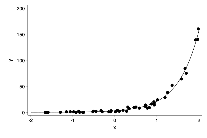
Poisson model
clear
set seed 39201
set obs 50
gen x=4*uniform()-2
local a=1
local b=2
gen linpred=`a'+`b'*x
gen y=rpoisson(exp(linpred))
poisson y x

twoway scatter  y x || function y= exp(_b[_cons] +_b[x]*x), ///
    range(-2 2) ylab(0(50)200) legend(off) ///
    ysc(fextend) xsc(fextend) lp(solid)
Iteration 0: log likelihood = -106.72731
Iteration 1: log likelihood = -99.820559
Iteration 2: log likelihood = -99.818201
Iteration 3: log likelihood = -99.818201
Poisson regression Number of obs = 50
LR chi2(1) = 2168.78
Prob > chi2 = 0.0000
Log likelihood = -99.818201 Pseudo R2 = 0.9157
─────────────┬────────────────────────────────────────────────────────────────
y │ Coef. Std. Err. z P>|z| [95% Conf. Interval]
─────────────┼────────────────────────────────────────────────────────────────
x │ 2.008777 .0572011 35.12 0.000 1.896665 2.12089
_cons │ 1.035443 .0922113 11.23 0.000 .8547122 1.216174
─────────────┴────────────────────────────────────────────────────────────────
──────────────────────────────────────────────
Coef.
──────────────────────────────────────────────
y
x 2.0 (0.1)
Intercept 1.0 (0.1)
──────────────────────────────────────────────
Standard errors in parentheses
Fig 15-1
Overdispersion and underdispersion
Negative binomial model for overdispersion
clear
set seed 46201
qui set obs 50
gen x=4*uniform()-2
local a=1
local b=2
gen linpred=`a'+`b'*x
local i=1
foreach a of num .1 1 10    {
    set seed 5302
    cap drop xg xbg y
    local ia=1/`a'  // phi
    gen xg=rgamma(`ia',`a')
    gen xbg=exp(linpred)*xg
    gen y=rpoisson(xbg)
    qui nbreg y x

    twoway scatter  y x || function y= exp(_b[_cons] +_b[x]*x), ///
        range(-2 2) ylab(0(50)200) legend(off) sub("{&phi}=`ia'") ///
        ysc(fextend) xsc(fextend) lp(solid) name(fig15_2_`i++',replace)

}
graph combine fig15_2_3 fig15_2_2 fig15_2_1,row(1) ysize(2.4) iscale(*1.5)
qui graph export img/fig15_2_stata.png,replace
Fig 15-2
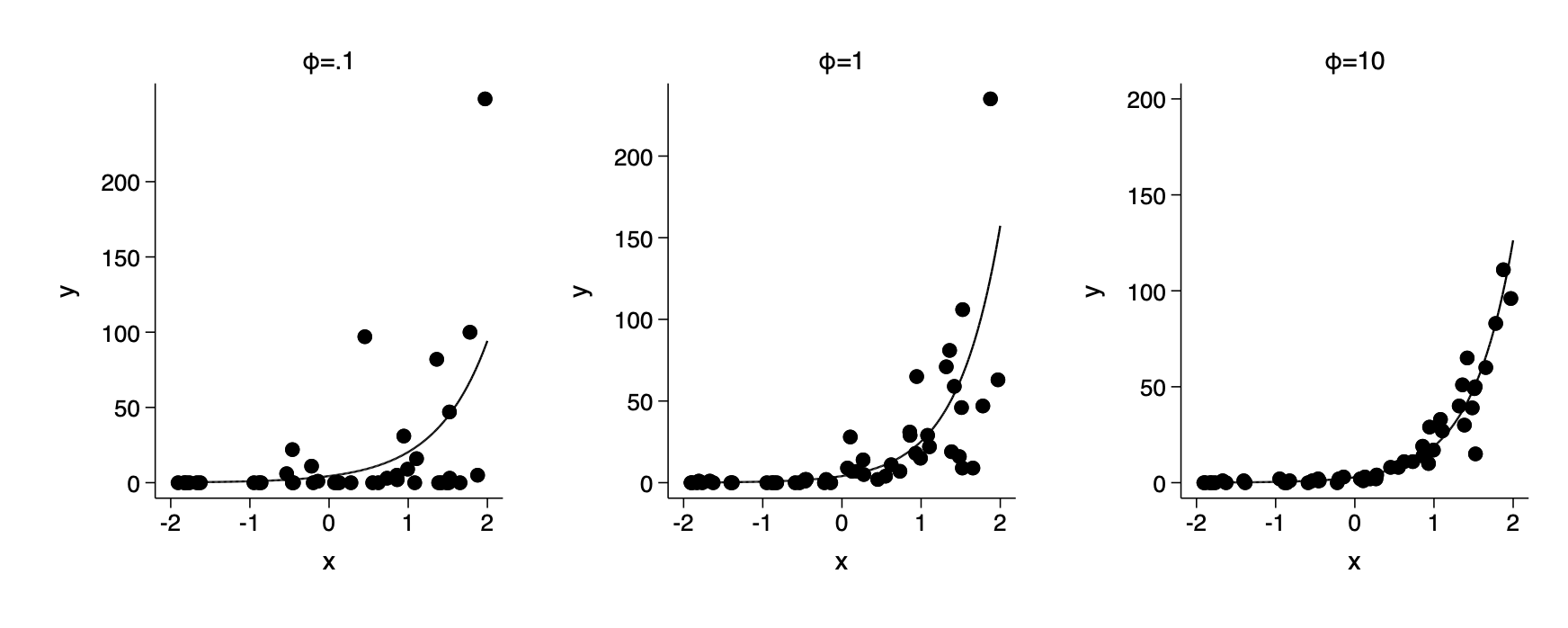
note - Gelman uses a different parameterization to simulate negative binomial observations from that required to use the built in random generating function rnbionomial. As a result we have to generate using a gamma mixture of poisson random variates. This is a small point and not worth losing sleep over. If you wanted to generate negative binomial observations you could use rnbionomial as shown in my simulation examples-part 1(at the bottom) from the bootstrap and simulation class
Interpreting Poisson or negative binomial regression coefficients
Exposure
Including log(exposure as a predictor in a Poisson or negative binomial regression)
Differences between the binomial and Poisson or NegBin models
Example: zeroes in count data
import delimited https://raw.githubusercontent.com/avehtari/ROS-Examples/master/Roaches/data/roaches.csv,clear
gen roach100=roach1/100
nbreg y roach100 treatment senior, exposure(exposure2)
Negative binomial regression Number of obs = 262
LR chi2(3) = 58.37
Dispersion = mean Prob > chi2 = 0.0000
Log likelihood = -889.29173 Pseudo R2 = 0.0318
─────────────┬────────────────────────────────────────────────────────────────
y │ Coef. Std. Err. z P>|z| [95% Conf. Interval]
─────────────┼────────────────────────────────────────────────────────────────
roach100 │ 1.288169 .2474593 5.21 0.000 .803158 1.77318
treatment │ -.7767854 .2450094 -3.17 0.002 -1.256995 -.2965758
senior │ -.3443717 .2616811 -1.32 0.188 -.8572572 .1685137
_cons │ 2.838781 .2290851 12.39 0.000 2.389782 3.287779
ln(exposu~2) │ 1 (exposure)
─────────────┼────────────────────────────────────────────────────────────────
/lnalpha │ 1.293662 .0954842 1.106516 1.480807
─────────────┼────────────────────────────────────────────────────────────────
alpha │ 3.646113 .3481463 3.023806 4.396494
─────────────┴────────────────────────────────────────────────────────────────
LR test of alpha=0: chibar2(01) = 1.0e+04 Prob >= chibar2 = 0.000
Stata’s negative binomial regression reports log(alpha) instead of phi so we have to calculate phi to get the same output as Gelman. We can do this using the nlcom command that calculates non-linear transformations of estimates and their accompanying standard errors. Then we add those results to the esttab output.
nlcom 1/(exp(_b[/lnalpha]))
estadd scalar reciprocal_disp=r(b)[1,1]
estadd scalar rd_std_error=r(V)[1,1]^.5
esttab,b(2) se wide mtitle("Coef.") drop(lnalpha:_cons) ///
    stats(reciprocal_disp rd_std_error)  ///
    coef(_cons "Intercept" ) nonum noobs nostar var(20)
──────────────────────────────────────────────
Coef.
──────────────────────────────────────────────
y
roach100 1.29 (0.25)
treatment -0.78 (0.25)
senior -0.34 (0.26)
Intercept 2.84 (0.23)
──────────────────────────────────────────────
reciprocal_disp 0.27
rd_std_error 0.03
──────────────────────────────────────────────
Standard errors in parentheses
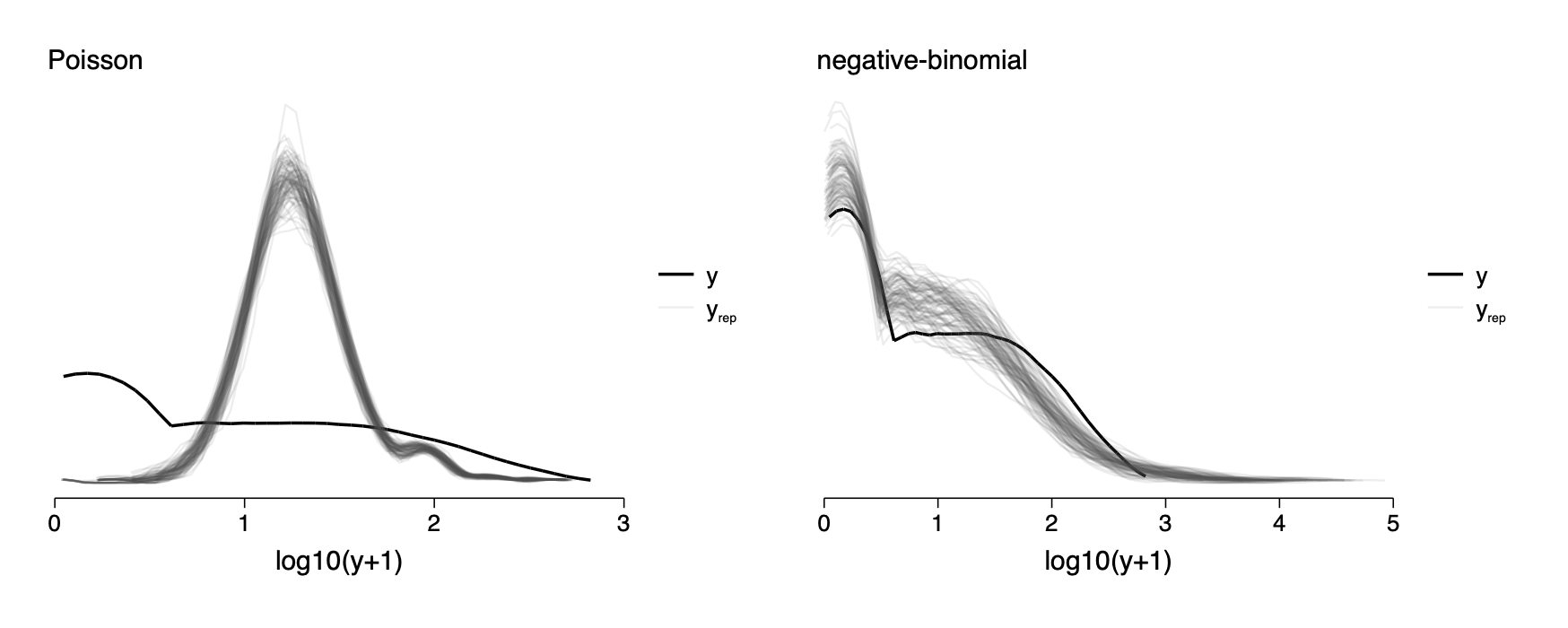
Checking model fit by comparing the data, y, to replicated datasets yrep
. gen log_y=log10(y+1)
***negative binomial model

qui nbreg y roach100 treatment senior, exposure(exposure2)
predict xb,xb

kdensity log_y, bw(.27) generate(newx0 kd_log_y0) nogr
gen log_y_r=.
gen pct_zero=.
forval i=1/100    {
    cap drop xg
    gen xg=rgamma(1/exp(_b[/lnalpha]),exp(_b[/lnalpha]))
    qui replace log_y_r=log10(rpoisson(exp(xb)*xg)+1)
    kdensity log_y_r,generate(newx`i' kd_log_y`i') nogr
}
preserve
reshape long kd_log_y newx,i(v1) j(rep)
sort rep newx
line kd_log_y newx if rep==0&newx>0,c(L) lp(solid) lc(black) lw(medthick) ///
    || line kd_log_y newx if rep>0&newx>0,c(L) lp(solid) lc(gs5%10) ///
    legend(label(1 "y") label(2 "y{subscript:rep}") pos(3)) ///
    ysc(off) xlab(0(1)5) name(negbin,replace) xtitle("log10(y+1)") ///
    subtitle(negative-binomial,pos(11))
restore


graph combine poisson negbin,row(1) ysize(2.4) iscale(*1.5)
cap drop xb
cap drop newx*
cap drop log_y_r
cap drop kd_log_y* ***Poisson model
qui poisson y roach100 treatment senior, exposure(exposure2)
predict xb,xb
kdensity log_y, bw(.27) generate(newx0 kd_log_y0) nogr
gen log_y_r=.
forval i=1/100 {
cap drop xg
qui replace log_y_r=log10(rpoisson(exp(xb))+1)
kdensity log_y_r,generate(newx`i' kd_log_y`i') nogr
}
preserve
reshape long kd_log_y newx,i(v1) j(rep)
sort rep newx
line kd_log_y newx if rep==0&newx>0,c(L) lp(solid) lc(black) lw(medthick) ///
|| line kd_log_y newx if rep>0&newx>0,c(L) lp(solid) lc(gs5%10) ///
legend(label(1 "y") label(2 "y{subscript:rep}") pos(3)) ///
ysc(off) xlab(0(1)3) name(poisson,replace) xtitle("log10(y+1)") ///
subtitle(Poisson,pos(11))
restoreFig 15-3
15.3 Logistic-binomial model
Rather than modeling as the unit of analysis a single trial that with an outcome that occurs or not, the logistic binomial model is for a count of the number of occurrences out of a specified number of trials.
To fit the logistic binomial model in stata you need to use the glm command which allows you to specify the dependent variable as a count of outcomes and a denominator for the number of trials.
. clear

. set obs 100
number of observations (_N) was 0, now 100

. gen height=rnormal(73,3)

. gen p=0.4+0.1*(height-72)/3

. gen numshots=20

. gen y=rbinomial(numshots,p)

. glm y height, family(binomial numshots)

Iteration 0:   log likelihood = -212.19839
Iteration 1:   log likelihood = -212.11004
Iteration 2:   log likelihood = -212.11004

Generalized linear models                         Number of obs   =        100
Optimization     : ML                             Residual df     =         98
                                                  Scale parameter =          1
Deviance         =  88.13073358                   (1/df) Deviance =   .8992932
Pearson          =  85.61122974                   (1/df) Pearson  =    .873584

Variance function: V(u) = u*(1-u/numshots)        [Binomial]
Link function    : g(u) = ln(u/(numshots-u))      [Logit]

                                                  AIC             =   4.282201
Log likelihood   = -212.1100377                   BIC             =  -363.1759

─────────────┬────────────────────────────────────────────────────────────────
             │                 OIM
           y │      Coef.   Std. Err.      z    P>|z|     [95% Conf. Interval]
─────────────┼────────────────────────────────────────────────────────────────
      height │   .1545549   .0160468     9.63   0.000     .1231037    .1860061
       _cons │  -11.48531   1.173959    -9.78   0.000    -13.78623   -9.184398
─────────────┴────────────────────────────────────────────────────────────────
The binomial model for count data
(skip)
Overdispersion
(skip)
Binary-data model
The more conventional form of logisitic regression. It is a special case of the logistic-binomial model with n=1.
Count-data model as a special case of the binary-data model
You can of course expand the logistic binomial model to have n trials for each observation. Then it is best to think of it as a multilevl model.
15.4 Probit regression: normally distributed data
There really is not much to choose between logit and probit models and almost no one uses probit models.
Instead of a logistic function to linearize the data it uses a cumulative normal distribution function - which is also sigmoid shaped running from 0 to 1.
15.5 Ordered and unordered categorical regression.
The ordered multinomial model
Latent variable model with cutpoints
Example of ordered categorical regression
Build dataset
. clear

. tempfile storable

. qui import delimited https://raw.githubusercontent.com/avehtari/ROS-Examples/master/Stor
> able/data/2playergames.csv,clear

. save `storable',replace
(note: file /var/folders/x6/yxhnms7s2xj76d9d7nrtfxk00000gn/T//S_00405.000001 not found)
file /var/folders/x6/yxhnms7s2xj76d9d7nrtfxk00000gn/T//S_00405.000001 saved

. qui import delimited https://raw.githubusercontent.com/avehtari/ROS-Examples/master/Stor
> able/data/3playergames.csv,clear

. append using `storable'

. save `storable',replace
file /var/folders/x6/yxhnms7s2xj76d9d7nrtfxk00000gn/T//S_00405.000001 saved

. qui import delimited https://raw.githubusercontent.com/avehtari/ROS-Examples/master/Stor
> able/data/6playergames.csv,clear

. append using `storable'

. l  in 1/6 ,c noobs

  ┌───────────────────────────────────────────────────────────────────────┐
  │ sch~l   per~n   round   pro~l   value   vote   cut~12   cu~23   sdl~t │
  ├───────────────────────────────────────────────────────────────────────┤
  │     1     101       1       1      16      1   32.835   58.75   1.103 │
  │     1     101       2       1      23      1   32.835   58.75   1.103 │
  │     1     101       3       1      63      3   32.835   58.75   1.103 │
  │     1     101       4       1      98      3   32.835   58.75   1.103 │
  │     1     101       5       1      16      1   32.835   58.75   1.103 │
  ├───────────────────────────────────────────────────────────────────────┤
  │     1     101       6       1      36      2   32.835   58.75   1.103 │
  └───────────────────────────────────────────────────────────────────────┘
Look at ordered logistic regression for person 401
. l vote value if person==401 in 1830/1835

      ┌──────────────┐
      │ vote   value │
      ├──────────────┤
1830. │    2      40 │
1831. │    1       4 │
1832. │    3      44 │
1833. │    1      23 │
1834. │    3      99 │
      ├──────────────┤
1835. │    2      82 │
      └──────────────┘

. ologit vote value if person==401

Iteration 0:   log likelihood = -21.921347
Iteration 1:   log likelihood = -11.505156
Iteration 2:   log likelihood =  -10.65744
Iteration 3:   log likelihood = -10.577739
Iteration 4:   log likelihood = -10.577675
Iteration 5:   log likelihood = -10.577675

Ordered logistic regression                     Number of obs     =         20
                                                LR chi2(1)        =      22.69
                                                Prob > chi2       =     0.0000
Log likelihood = -10.577675                     Pseudo R2         =     0.5175

─────────────┬────────────────────────────────────────────────────────────────
        vote │      Coef.   Std. Err.      z    P>|z|     [95% Conf. Interval]
─────────────┼────────────────────────────────────────────────────────────────
       value │   .1254895   .0413897     3.03   0.002     .0443672    .2066119
─────────────┼────────────────────────────────────────────────────────────────
       /cut1 │   4.175663   1.692034                      .8593386    7.491988
       /cut2 │   8.418933   2.834125                       2.86415    13.97372
─────────────┴────────────────────────────────────────────────────────────────
Given the small number of observations the ordered logistic regression here is somewhat different from the bayesian ordered logistic regression illustrated in the text book.
We can show this within R
    vote value factor_vote
300    2    40           2
301    1     4           1
302    3    44           3
303    1    23           1
304    3    99           3
305    2    82           2
Using the bayesian ordered logistic regression we get the same results as the textbook.
> fit_1 <- stan_polr(factor_vote ~ value, data = data_401,
+                prior = R2(0.3, "mean"), refresh = 0)
> print(fit_1, digits=2)
stan_polr
 family:       ordered [logistic]
 formula:      factor_vote ~ value
 observations: 20
------
      Median MAD_SD
value 0.09   0.03

Cutpoints:
    Median MAD_SD
1|2 2.75   1.40
2|3 5.94   2.21

------
* For help interpreting the printed output see ?print.stanreg
* For info on the priors used see ?prior_summary.stanreg
>
But using regular ordered logistic regession in R we get exactly the same as what we got using Stata above.
> require(MASS)
> require(Hmisc)
> polr(factor_vote ~ value, data = data_401,start=c(1,1,2))
Call:
polr(formula = factor_vote ~ value, data = data_401, start = c(1,
    1, 2))

Coefficients:
    value
0.1254895

Intercepts:
     1|2      2|3
4.175663 8.418932

Residual Deviance: 21.15535
AIC: 27.15535