—
Gelman Chapter 13 examples
21 Oct 2020
Use for outputs
local gelman_output esttab,b(1) se wide mtitle("Coef.") scalars("rmse sigma") ///
    coef(_cons "Intercept" rmse "sigma") nonum noobs nostar var(15)
local gelman_output2 esttab,b(2) se wide mtitle("Coef.") scalars("rmse sigma") ///
    coef(_cons "Intercept" rmse "sigma") nonum noobs nostar var(15)
Chapter 13
13.1 Logistic regression with single predictor
- Example: modeling political preference given income
use "https://github.com/avehtari/ROS-Examples/blob/master/NES/data/nes5200_processed_voters_realideo.dta?raw=true"
keep if !missing(black,female,educ1,age,income,state)
keep if year>=1952
gen dvote=presvote==1
gen rvote=presvote==2
keep if !missing(rvote,dvote)&(rvote==1|dvote==1)
logit rvote income if year==1992
─────────────────────────────────────────
Coef.
─────────────────────────────────────────
rvote
income 0.3 (0.1)
Intercept -1.4 (0.2)
─────────────────────────────────────────
sigma
─────────────────────────────────────────
Standard errors in parentheses
- The logistic regression model problem of 0 and 1 bounding logic is compressed at ends of probability scale
- Fitting the model using stan_glm and displaying uncertainty in the fitted model
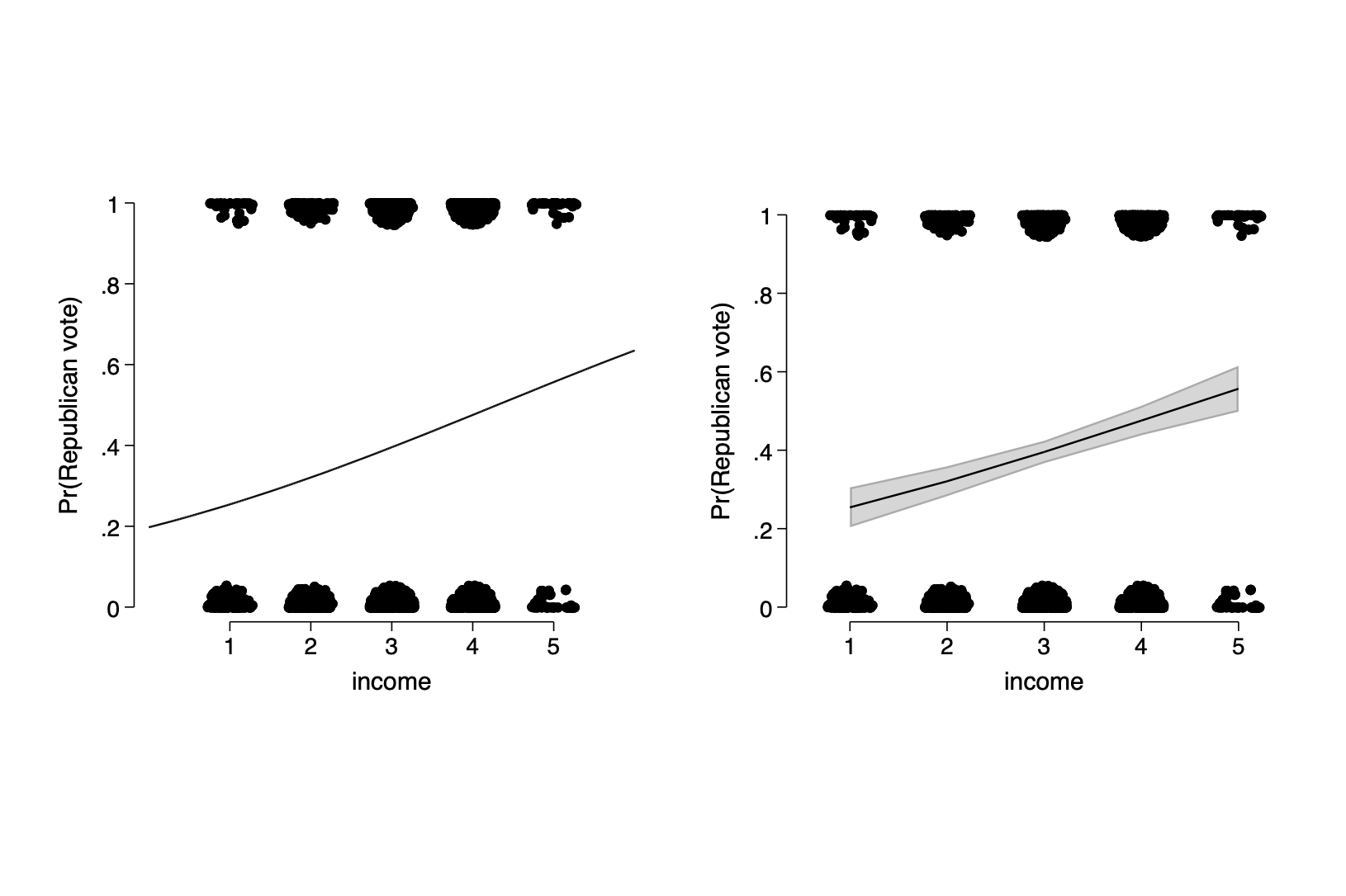
* Figure 13.2
twoway (function y=invlogit(_b[_cons]+_b[income]*x),range(0 6)) ///
    (scatter rvote income,jitter(5) ms(o)),  graphregion(margin(t=25 b=25)) ///
    xlab(1(1)5) xtitle(income) ytitle("Pr(Republican vote)") ///
    name(a132,replace) legend(off)
qui margins, at(income=(1(1)5))
marginsplot ,ciopt(color(black%20) ) plotopt(ms(i) legend(off) ) xtitle(income) ///
    nolabel recastci(rarea) title(" ") graphregion(margin(t=20 b=25))  ///
    name(b132,replace) ytitle("Pr(Republican vote)") ///
    addplot(scatter rvote income,jitter(5) ms(o) xscale(range(0.5 5.5)))
graph combine a132 b132, ycommon
Figure 13.2
13.2 Interpreting logistic regression coefficients and the divide by 4 rule
- Evaluation at and near the mean of the data
. qui sum income

. di invlogit(-1.40 + 0.33*r(mean))
.40409988

. di invlogit(_b[_cons] + _b[income]*r(mean))
.40063528
- The divide-by-4 rule
- Interpretation of coefficients as odds ratios
- Coefficient estimates and standard errors
- Statistical significance
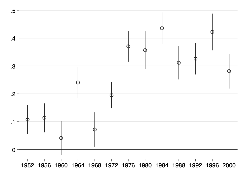
- Displaying the results of several logistic regressions
local i=1
forval year=1952(4)2000    {
    qui logit rvote income if year==`year'
    est store m`i++'
    }
coefplot (m* ), drop(_cons rvote)  aseq swapnames vertical ///
        coeflabels(m1 = "1952" m2= "1956" m3= "1960" m4= "1964" ///
                    m5= "1968" m6= "1972" m7= "1976" m8= "1980" ///
                    m9= "1984" m10= "1988" m11= "1992" m12= "1996" ///
                    m13= "2000") yline(0) levels(68)
Figure 13.4
13.3 Predictions and comparisons
- Can predict a probability for a new point
- point prediction using predict, person with income=5
. di invlogit(-1.40+0.33*5)
.5621765
- linear prediction with uncertainty using posterior_linpred maximum likelihood equivalent using margins
. qui logit rvote income if year==1992

. margins ,predict(xb) at(income=5)  noatlegend

Adjusted predictions                            Number of obs     =      1,179
Model VCE    : OIM

Expression   : Linear prediction (log odds), predict(xb)

─────────────┬────────────────────────────────────────────────────────────────
             │            Delta-method
             │     Margin   Std. Err.      z    P>|z|     [95% Conf. Interval]
─────────────┼────────────────────────────────────────────────────────────────
       _cons │   .2278436   .1208307     1.89   0.059    -.0089802    .4646674
─────────────┴────────────────────────────────────────────────────────────────
- Expected outcome with uncertainty using posterior_epred maximum likelihood equivalent using margins
. margins, at(income=5)  noatlegend

Adjusted predictions                            Number of obs     =      1,179
Model VCE    : OIM

Expression   : Pr(rvote), predict()

─────────────┬────────────────────────────────────────────────────────────────
             │            Delta-method
             │     Margin   Std. Err.      z    P>|z|     [95% Conf. Interval]
─────────────┼────────────────────────────────────────────────────────────────
       _cons │   .5567158    .029819    18.67   0.000     .4982716    .6151599
─────────────┴────────────────────────────────────────────────────────────────
predictive distribution for a new observation using posterior_predict N/A only applies for bayesian est.
prediction given a range of input values
. margins, at(income=(1(1)5)) noatlegend

Adjusted predictions                            Number of obs     =      1,179
Model VCE    : OIM

Expression   : Pr(rvote), predict()

─────────────┬────────────────────────────────────────────────────────────────
             │            Delta-method
             │     Margin   Std. Err.      z    P>|z|     [95% Conf. Interval]
─────────────┼────────────────────────────────────────────────────────────────
         _at │
          1  │   .2542381   .0259236     9.81   0.000     .2034288    .3050474
          2  │   .3207907   .0194448    16.50   0.000     .2826795    .3589019
          3  │   .3955251   .0145538    27.18   0.000     .3670002    .4240501
          4  │   .4754819   .0191849    24.78   0.000     .4378802    .5130836
          5  │   .5567158    .029819    18.67   0.000     .4982716    .6151599
─────────────┴────────────────────────────────────────────────────────────────
We can't calculate the probability that Bush was more popular in people with
income level 5 than those with  income level 4, but we can calculate the
difference in average probability.
. margins, at(income=(1(1)5)) contrast(atcontrast(rb5._at)) noatlegend
Contrasts of adjusted predictions Number of obs = 1,179
Model VCE : OIM
Expression : Pr(rvote), predict()
─────────────┬──────────────────────────────────
│ df chi2 P>chi2
─────────────┼──────────────────────────────────
_at │
(1 vs 5) │ 1 37.72 0.0000
(2 vs 5) │ 1 34.36 0.0000
(3 vs 5) │ 1 33.12 0.0000
(4 vs 5) │ 1 34.09 0.0000
Joint │ 2 87.86 0.0000
─────────────┴──────────────────────────────────
─────────────┬────────────────────────────────────────────────
│ Delta-method
│ Contrast Std. Err. [95% Conf. Interval]
─────────────┼────────────────────────────────────────────────
_at │
(1 vs 5) │ -.3024777 .0492497 -.3990052 -.2059501
(2 vs 5) │ -.2359251 .0402454 -.3148046 -.1570455
(3 vs 5) │ -.1611906 .028009 -.2160872 -.106294
(4 vs 5) │ -.0812339 .0139129 -.1085025 -.0539652
─────────────┴────────────────────────────────────────────────
- Logistic regression with just an intercept using classical standard error (approximation) 50 people, 10 with disease 0.20 ± sqrt((0.2*0.8)/50) = 0.06
. di "[" 0.20 - sqrt((0.2*0.8)/50) "," 0.20 + sqrt((0.2*0.8)/50) "]"
[.14343146,.25656854]
or:
clear
set obs 50
gen y=(_n<11)
logit y
di invlogit(_b[_cons])
di "[" invlogit(_b[_cons]-_se[_cons]) "," invlogit(_b[_cons]+_se[_cons]) "]"
number of observations (_N) was 0, now 50
─────────────────────────────────────────
Coef.
─────────────────────────────────────────
y
Intercept -1.39 (0.35)
─────────────────────────────────────────
sigma
─────────────────────────────────────────
Standard errors in parentheses
. di invlogit(_b[_cons])
.2

. di "[" invlogit(_b[_cons]-_se[_cons]) "," invlogit(_b[_cons]+_se[_cons]) "]"
[.14933227,.26255306]
or:
. margins,level(68) // CI changed for +/- 1 s.d.
Warning: prediction constant over observations.

Predictive margins                              Number of obs     =         50
Model VCE    : OIM

Expression   : Pr(y), predict()

─────────────┬────────────────────────────────────────────────────────────────
             │            Delta-method
             │     Margin   Std. Err.      z    P>|z|     [68% Conf. Interval]
─────────────┼────────────────────────────────────────────────────────────────
       _cons │         .2   .0565685     3.54   0.000      .143745     .256255
─────────────┴────────────────────────────────────────────────────────────────
- Logistic regression with single binary predictor
clear
set obs 110
gen pop_b=(_n>50)
gen test_pos=(_n<=10)|(_n>50&_n<=70)
logit test_pos i.pop_b
margins pop_b
* now the difference in probabilities for the two groups
margins r.pop_b
number of observations (_N) was 0, now 110
─────────────────────────────────────────
Coef.
─────────────────────────────────────────
test_pos
0.pop_b 0.00 (.)
1.pop_b 0.69 (0.45)
Intercept -1.39 (0.35)
─────────────────────────────────────────
sigma
─────────────────────────────────────────
Standard errors in parentheses
Adjusted predictions Number of obs = 110
Model VCE : OIM
Expression : Pr(test_pos), predict()
─────────────┬────────────────────────────────────────────────────────────────
│ Delta-method
│ Margin Std. Err. z P>|z| [95% Conf. Interval]
─────────────┼────────────────────────────────────────────────────────────────
pop_b │
0 │ .2 .0565685 3.54 0.000 .0891277 .3108723
1 │ .3333333 .0608581 5.48 0.000 .2140537 .4526129
─────────────┴────────────────────────────────────────────────────────────────
Contrasts of adjusted predictions Number of obs = 110
Model VCE : OIM
Expression : Pr(test_pos), predict()
─────────────┬──────────────────────────────────
│ df chi2 P>chi2
─────────────┼──────────────────────────────────
pop_b │ 1 2.58 0.1086
─────────────┴──────────────────────────────────
─────────────┬────────────────────────────────────────────────
│ Delta-method
│ Contrast Std. Err. [95% Conf. Interval]
─────────────┼────────────────────────────────────────────────
pop_b │
(1 vs 0) │ .1333333 .0830885 -.0295172 .2961839
─────────────┴────────────────────────────────────────────────
13.4 Latent data formulation
Read but no examples
13.5 (skip)Maximum Likelihood and Bayesian inference for logistic regression
13.6 (skip)Cross validation and log score for logistic regression
13.7 Building a logistic regression model: wells in Bangladesh
Logistic regression with just one predictor
import delimited using "https://raw.githubusercontent.com/avehtari/ROS-Examples/master/Arsenic/data/wells.csv", clear
logit switch dist
est store one_var
*gen dist100=dist/100  // variable already in dataset
logit switch dist100
est store one_var_c
─────────────────────────────────────────
Coef.
─────────────────────────────────────────
switch
dist -0.006 (0.001)
Intercept 0.606 (0.060)
─────────────────────────────────────────
sigma
─────────────────────────────────────────
Standard errors in parentheses
─────────────────────────────────────────
Coef.
─────────────────────────────────────────
switch
dist100 -0.6 (0.1)
Intercept 0.6 (0.1)
─────────────────────────────────────────
sigma
─────────────────────────────────────────
Standard errors in parentheses
Graphing the fitted model
Plotting centered variables with marginsplot doesn’t easily give you the x axis scale you want (0-350) although you can relabel with a bit of work
qui logit switch dist
hist dist,freq xtitle("Distance (in meters) to the nearest safe well") ///
    name(fig13_8a,replace)
margins, at(dist=(0(50)300))
marginsplot ,noci plotopt(ms(i) legend(off) ) xtitle(Distance) ///
    nolabel  title(" ")   ///
    ytitle("Pr(Switch)") name(fig13_8b,replace) ///
    addplot(scatter switch dist,jitter(7) ms(p)  ///
    xscale(range(0.5 5.5)))
Figure 13.8

Adding a second input variable
hist arsenic, freq xtitle("Arsenic concentration in well water")Figure 13.9

Instead of using the leave-out-one log score for comparing models we use a likelihood ratio test of nested models. This compares the log likelihoods of the two models.
logit switch dist100 arsenic
est store two_var_c
lrtest two_var_c one_var_c
─────────────────────────────────────────
Coef.
─────────────────────────────────────────
switch
dist100 -0.90 (0.10)
arsenic 0.46 (0.04)
Intercept 0.00 (0.08)
─────────────────────────────────────────
sigma
─────────────────────────────────────────
Standard errors in parentheses
Likelihood-ratio test LR chi2(1) = 145.57
(Assumption: one_var_c nested in two_var_c) Prob > chi2 = 0.0000
The likelihood test is significant which suggest that the log likelhood has improved with the addition of the second predictor.
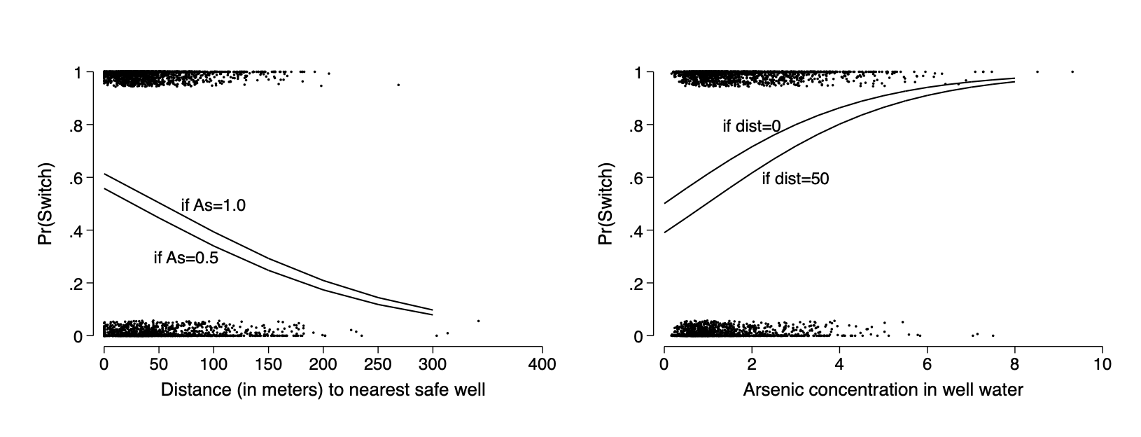
Graphing the fitted model with two predictors
logit switch c.dist c.arsenic
margins ,at(dist=(0(50)300) arsenic=(0.5 1.0))
marginsplot ,noci plotopt(ms(i) legend(off) )     nolabel  title(" ") ///
    xtitle("Distance (in meters) to nearest safe well") ///
    ytitle("Pr(Switch)") name(fig13_10a,replace) ///
    addplot(scatter switch dist,jitter(7) ms(p))  ///
    text(.5 100 "if As=1.0") text(0.3 75 "if As=0.5")
margins ,at(arsenic=(0(.5)8) dist=(0 50))
marginsplot ,noci plotopt(ms(i) legend(off)) nolabel  title(" ") ///
    xtitle("Arsenic concentration in well water") xlab(0(2)8) ///
    ytitle("Pr(Switch)") name(fig13_10b,replace) ylab(0(.2)1) ///
    text(.8 2 "if dist=0") text(0.6 3 "if dist=50")     ///
    addplot(scatter switch arsenic,jitter(7) ms(p))
graph combine fig13_10a fig13_10b ,ysize(2.3) iscale(*1.5)
Figure 13.10