—
Under construction
Gelman Chapter 14 examples
5 Nov 2020
Use for outputs
local gelman_output esttab,b(1) se wide mtitle("Coef.") scalars("rmse sigma") ///
    coef(_cons "Intercept" rmse "sigma") nonum noobs nostar var(20)
local gelman_output2 esttab,b(2) se wide mtitle("Coef.") scalars("rmse sigma") ///
    coef(_cons "Intercept" rmse "sigma") nonum noobs nostar var(20)
Chapter 14
14.1 Graphing logistic regression and binary data
One predictor
clear
set seed 7008
set obs 50
local a=2
local b=3
local x_mean=-`a'/`b'
local x_sd=4/`b'
gen x=rnormal(`x_mean',`x_sd')
gen y=rbinomial(1,invlogit(`a'+`b'*x))
logit y x
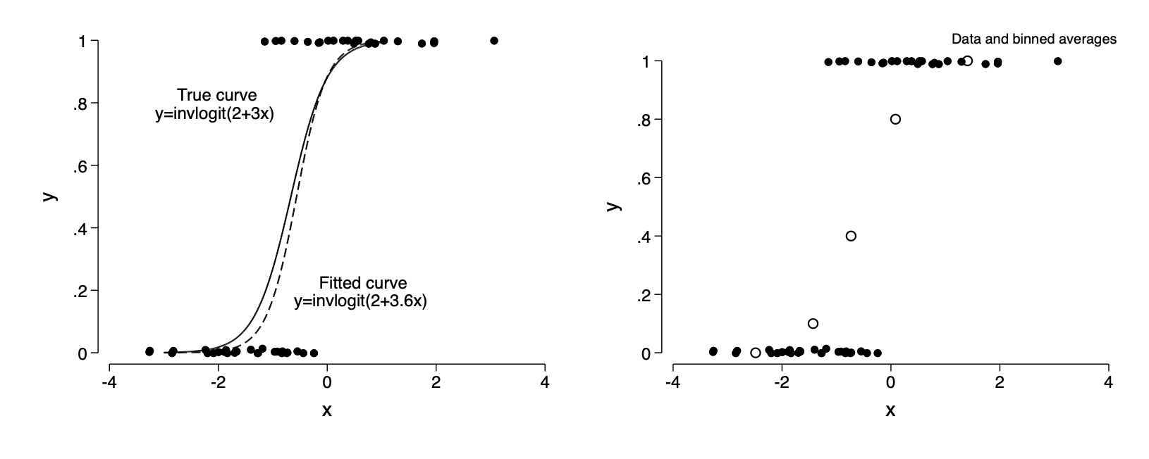
twoway (function y=invlogit(2+3*x),range(-3 1)) ///
(function y=invlogit(_b[_cons]+_b[x]*x), range(-3 1)) ///
(scatter y x,jitter(2) ms(o) ) , legend(off) ///
text(.2 -.75 "Fitted curve" "y=invlogit(2+3.6x) ", placement(e)) ///
text(.8 -.75 "True curve" "y=invlogit(2+3x) ", placement(w)) name(f14_1a,replace)binscatter y x, nq(5) savedata(binned,replace)
preserve
insheet using binned.csv,clear
tempname binned
save `binned',replace
restore
append using `binned', gen(binned)
twoway (scatter y x if binned==1, ms(Oh)) ///
(scatter y x if binned==0,jitter(2) ms(o) ),legend(off) ///
note(Data and binned averages,pos(1)) name(f14_1b,replace)graph combine f14_1a f14_1b, ysize(2.4) iscale(*1.5)*graph export img/fig14_1.png,replaceFigure 14.1
Two predictors
clear
set seed 38832
set obs 50
local a=2
local b=3
local b2=4
gen x1=rnormal(0,0.4)
gen x2=rnormal(-0.5,0.4)
gen y=rbinomial(1,invlogit(`a'+`b'*x1+`b2'*x2))
logit y x1 x2
* Pr(y=1)=0.5 when a+bx1+b2x2=logit(.5)=0 or x2=-a/b2-(b/b2)
* Pr(y=1)=0.9 when a+bx1+b2x2=logit(.9)=2.2 or x2=-a/b2-(b/b2)-2.2/b2
twoway (function y=-_b[_cons]/_b[x2]-(_b[x1]/_b[x2])*x,range(-1 1)) ///
    (function y=-_b[_cons]/_b[x2]-(_b[x1]/_b[x2])*x-logit(.9)/_b[x2] ///
    ,range(-1 1) )  ///
    (function y=-_b[_cons]/_b[x2]-(_b[x1]/_b[x2])*x-logit(.1)/_b[x2] ///
    ,range(-1 1) lpattern(dash) )  ///
    (scatter x2 x1 if y==1) (scatter x2 x1 if y==0), ///
    xtitle(x1) ytitle(x2) legend(off)
* graph export img/fig14_2.png,replaceFigure 14.2

The dotted lines represent variation inherent in the binomial
14.2 Logistic regression with interactions
- Intro Return to well switching data
import delimited using "https://raw.githubusercontent.com/avehtari/ROS-Examples/master/Arsenic/data/wells.csv", clear
*gen dist100=dist/100  // variable already in dataset
logit switch c.dist100##c.arsenic
cap confirm file data/wells.dta
if _rc {
import delimited using "https://raw.githubusercontent.com/avehtari/ROS-Examples/master/Arsenic/data/wells.csv", clear
save data/wells
}
else use data/wells.dta,clear
qui logit switch c.dist100##c.arsenic
`gelman_output2'- Centering the input variables
- re-fitting using centered inputs
sum dist100,meanonly
gen c_dist100=dist100-r(mean)
sum arsenic,meanonly
gen c_arsenic=arsenic-r(mean)
logit switch c.c_dist100##c.c_arsenic
est store interaction_model
sum dist100,meanonly
gen c_dist100=dist100-r(mean)
sum arsenic,meanonly
qui gen c_arsenic=arsenic-r(mean)
qui logit switch c.c_dist100##c.c_arsenic
est store interaction_model
`gelman_output2'- statistical significance of the interaction
qui logit switch c.c_dist100 c.c_arsenic
est store base_model
lrtest base_model interaction_model
qui logit switch c.c_dist100 c.c_arsenic
est store base_model
lrtest base_model interaction_modelR code
library("rstanarm")
library("loo")
library("haven")
wells <- read_dta("data/wells.dta")
wells$dist100<-wells$dist/100
fit_4<-stan_glm(switch ~ dist100 + arsenic + dist100:arsenic,family=binomial(link="logit"), data=wells)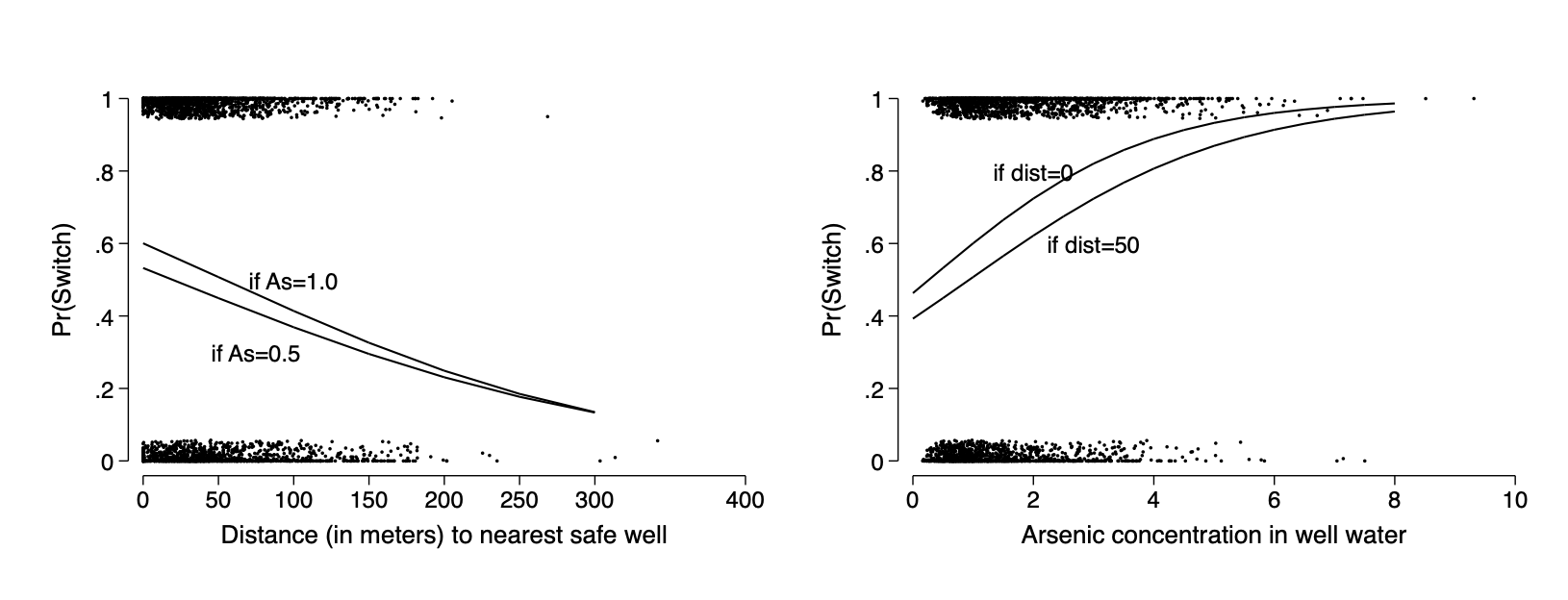
loo(fit_4)- graphing the model with interactions
Note that both the centering and dividing distance by 100 were mainly for ease of interpreation of the coefficients.
Since they are linear transformations they do not change the model in any substantive way and when using marginsplot it is a lot easier to graph the variables on their natural scale if you make the model using that scale.
qui logit switch c.dist##c.arsenic
margins ,at(dist=(0(50)300) arsenic=(0.5 1.0))
marginsplot ,noci plotopt(ms(i) legend(off) )     nolabel  title(" ") ///
    xtitle("Distance (in meters) to nearest safe well") ///
    ytitle("Pr(Switch)") name(fig14_3a,replace) ///
    addplot(scatter switch dist,jitter(7) ms(p))  ///
    text(.5 100 "if As=1.0") text(0.3 75 "if As=0.5")
margins ,at(arsenic=(0(.5)8) dist=(0 50))
marginsplot ,noci plotopt(ms(i) legend(off)) nolabel  title(" ") ///
    xtitle("Arsenic concentration in well water") xlab(0(2)8) ///
    ytitle("Pr(Switch)") name(fig14_3b,replace) ylab(0(.2)1) ///
    text(.8 2 "if dist=0") text(0.6 3 "if dist=50")     ///
    addplot(scatter switch arsenic,jitter(7) ms(p))
graph combine fig14_3a fig14_3b ,ysize(2.3) iscale(*1.5)
*graph export img/fig14_3.png,replaceFigure 14.2
- adding social predictors
*gen educ4=educ/4 // already defined
logit switch c.dist100 c.arsenic educ4 assoc
logit switch c.dist100 c.arsenic educ4
est store social
lrtest social base_model
*gen educ4=educ/4 // already defined
qui logit switch c.dist100 c.arsenic educ4 assoc
`gelman_output2'
qui logit switch c.dist100 c.arsenic educ4
`gelman_output2'
est store social
lrtest social base_model- adding further interactions
sum educ4,meanonly
gen c_educ4=educ4-r(mean)
qui logit switch educ4 c_dist10 c_arsenic c.c_arsenic#c.c_educ4  c.c_dist100#c.c_educ4
`gelman_output2'
lrtest . social
qui sum educ4,meanonly
qui gen c_educ4=educ4-r(mean)
qui logit switch educ4 c_dist10 c_arsenic c.c_arsenic#c.c_educ4 c.c_dist100#c.c_educ4
est store p246_model
`gelman_output2'
lrtest . social Gelman uses centered education in the interactions but not in the main effect so you have to specify the interactions separately.
Note if you want to refer to the last model estimated without giving it a name you can just use the “.” in the lrtest commmand
- standardizing predictors
14.3 Predictive simulation
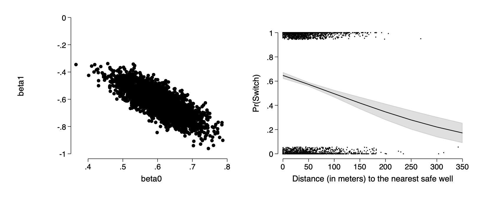
- simulating uncertainty in the coefficients
In regular GLM estimation we don’t use simulation in fitting the model but we can describe the uncertainty in the estimated coefficients using the s.e. of the coefficients and the variance-covariance matrix
qui logit switch dist100
cap drop beta0 beta1
mat m=(_b[dist], _b[_cons])
mat sd=(_se[dist], _se[_cons])
mat C=corr(e(V))
drawnorm beta1 beta0, means(m) sds(sd)  corr(C)
scatter beta1 beta0,ms(o) ylab(-1(.2)0) name(f14_4a,replace)

logit switch dist
margins, at(dist=(0(50)350))
marginsplot ,plotopt(ms(i) legend(off) ) xtitle(Distance) ///
    nolabel  title(" ")  recastci(rarea) ciopts(astyle(ci) acolor(%50)) ///
    xtitle("Distance (in meters) to the nearest safe well") ///
    ytitle("Pr(Switch)")  name(f14_4b,replace) ///
    addplot(scatter switch dist,jitter(7) ms(p)  ///
    xlab(0(50)350) )
graph combine f14_4a f14_4b, ysize(2.5) iscale(*1.5)
qui logit switch dist100
cap drop beta0 beta1
mat m=(_b[dist], _b[_cons])
mat sd=(_se[dist], _se[_cons])
mat C=corr(e(V))
drawnorm beta1 beta0, means(m) sds(sd) corr(C)
* omit graph if done but generate beta0 beta1 for next section
* graph export img/fig14_4.png,replaceFigure 14.4
- predictive simulation using the binomial distribution
cap drop y1-y10
qui logit switch dist
set seed 32948
qui sum dist100
local dist_mean=r(mean)
local dist_sd=r(sd)
forval i=1/10     {
    qui gen y`i'=.
    local dist=rnormal(`dist_mean',`dist_sd')
    forval j=1/3020    {
        local test=rbinomial(1,invlogit(beta0+beta1*`dist'))
        qui replace y`i'=`test' in `j++'
        }
    local i=`i++'
    }
l beta0 beta1 y1 y2 y10 in -5/l,table
tabstat y1-y3 y10,stat(mean)
qui {
cap drop y1-y10
qui logit switch dist
set seed 32948
qui sum dist100
local dist_mean=r(mean)
local dist_sd=r(sd)
forval i=1/10 {
qui gen y`i'=.
local dist=rnormal(`dist_mean',`dist_sd')
forval j=1/3020 {
qui replace y`i'=rbinomial(1,invlogit(beta0+beta1*`dist')) in `j++'
}
local i=`i++'
}
}
l beta0 beta1 y1 y2 y10 in -5/l,table
tabstat y1-y3 y10,stat(mean)- predictive simulation using the latent logistic distribution
set seed 32948
qui sum dist100
local dist_mean=r(mean)
local dist_sd=r(sd)
forval i=1/10     {
    local dist=rnormal(`dist_mean',`dist_sd')
    forval j=1/3020    {
        local outcome=(beta0+beta1*`dist'+rlogistic())>0
        qui replace y`i'=`outcome' in `j++'
        }
    local i=`i++'
    }
l beta0 beta1 y1 y2 y10 in -5/l,table
tabstat y1-y3 y10,stat(mean)
qui {
set seed 32948
qui sum dist100
local dist_mean=r(mean)
local dist_sd=r(sd)
forval i=1/10 {
local dist=rnormal(`dist_mean',`dist_sd')
forval j=1/3020 {
local outcome=(beta0+beta1*`dist'+rlogistic())>0 // eqiv logit(uniform())
qui replace y`i'=`outcome' in `j++'
}
local i=`i++'
}
}
l beta0 beta1 y1 y2 y10 in -5/l,table
tabstat y1-y3 y10,stat(mean)The predictions are slightly different but would be the same on average
14.4 Average predictive comparisons on the probability scale
- problems with evaluating predictive comparisons at central value
- demonstration with the well-switching example
qui logit switch dist100 arsenic educ4
`gelman_output2'
margins ,at(dist=(1 0)) contrast(atcontrast(r)) noatlegend
margins ,at(arsenic=(0.5 1.0)) contrast(atcontrast(r)) noatlegend
margins ,at(educ=(0 3)) contrast(atcontrast(r)) noatlegend- average predictive comparisons in the presence of interactions
qui logit switch arsenic c.dist##c.educ4
margins,at(dist=(0 100)) contrast(atcontrast(r)) noatlegend
14.5 Residuals for discrete-data regression
- residuals and binned residuals
est restore p246_model
`gelman_output2'
predict prob_switch
gen resid=switch-prob_switch
scatter resid prob_switch, ytitle(Observed-estimated) title(Residual plot) ///
    ylab(-1(1)1) xlab(0(.2)1) xtitle("Estimated Pr(switching)") ms(p)
est restore p246_model
`gelman_output2'
qui predict prob_switch
qui gen resid=switch-prob_switch
scatter resid prob_switch, ytitle(Observed-estimated) ///
title(Residual plot) ylab(-1(1)1) xlab(0(.2)1) ///
xtitle("Estimated Pr(switching)") ms(p)
qui graph export img/fig14_8a.png,replace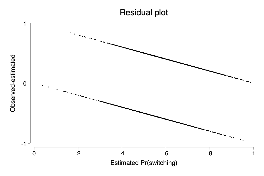
Two ways to get the binned residual plots
binscatter resid prob_switch,nq(40) savedata(binned) replace
clear
insheet using binned.csv,clear
gen std=sqrt(((prob_switch+resid)*(1-(prob_switch+resid)))/(3020/40))
gen low = -2*std
gen high= 2*std
twoway line low prob_switch || scatter resid prob_switch ///
    || line high prob_switch , name(bin1,replace) ///
    xtitle("Estimated Pr(switching)")
preserve
qui binscatter resid prob_switch,nq(40) savedata(binned) replace
clear
insheet using binned.csv,clear
gen std=sqrt(((prob_switch+resid)*(1-(prob_switch+resid)))/(3020/40))
gen low = -2*std
gen high= 2*std
twoway line low prob_switch || scatter resid prob_switch ///
|| line high prob_switch , name(bin1,replace) legend(off) ///
xtitle("Estimated Pr(switching)")
qui graph export img/fig14_8b1.png,replace
restore
drop prob_switch resid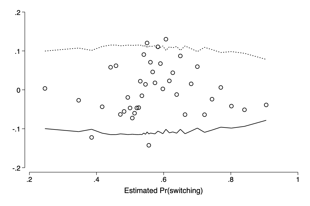
I have written a progam to create binned residual graphs
cap prog drop bin_resid
run  http://www-personal.umich.edu/~thofer/ado/bin_resid.do
est restore p246_model
bin_resid switch, pred(pred_switch) xtitle("Estimated Pr(switching)")
qui graph export img/fig14_8b2.png,replace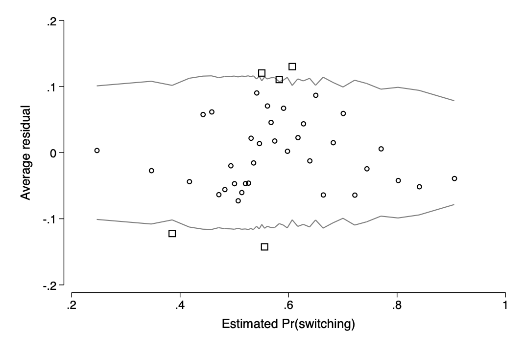
- plotting binned residuals versus inputs of interest
bin_resid switch dist, pred(pred_switch) name(f14_9a) ///
    xtitle("Distance to nearest safe well")
bin_resid switch arsenic, pred(pred_switch) name(f14_9b) ///
    xtitle(Arsenic level)
graph combine f14_9a f14_9b, ysize(2.5)  iscale(*1.5)
qui graph export img/fig14_9.png,replace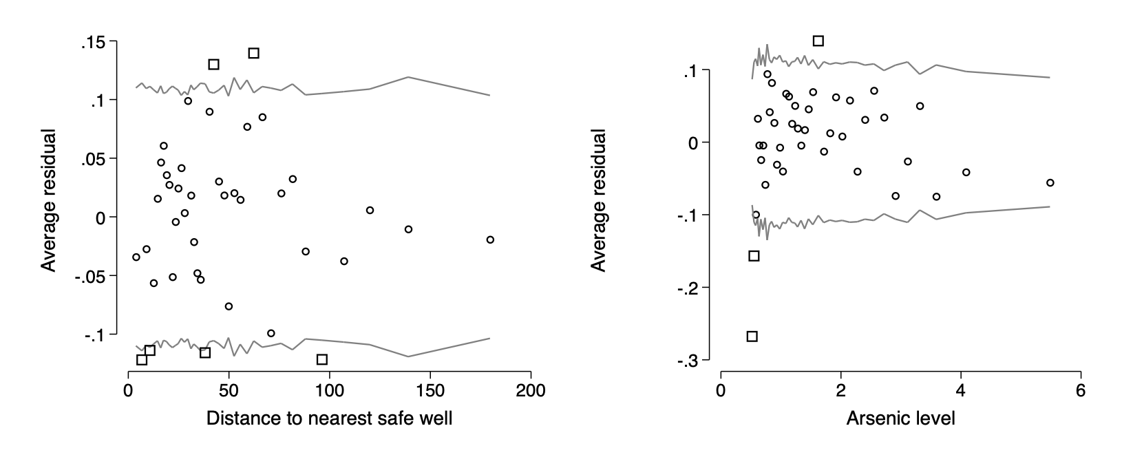
- improving a model by transformation
gen log_arsenic=log(arsenic)
sum log_arsenic,meanonly
gen c_log_arsenic=log_arsenic-r(mean)
qui logit switch c.c_dist100##c.c_educ4 c.c_log_arsenic##c.c_educ4
`gelman_output2'
bin_resid switch arsenic, pred(pred_switch) name(f14_10) ///
    xtitle(Arsenic level)
qui graph export img/fig14_10.png,name(f14_10) replace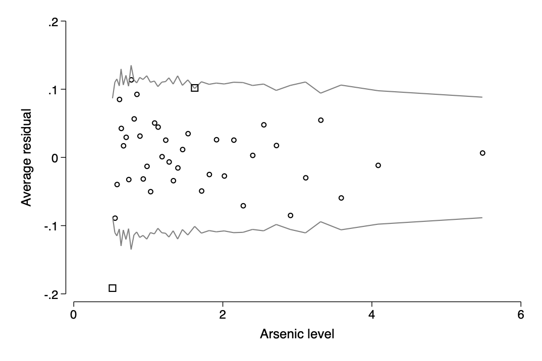
- error rate and comparison t the null model
- where error can mislead ## 14.6 Identification and separation
- complete separation
- weakly informative default